This page was generated from docs/basics/getting_started.ipynb.
Interactive online version:
Introduction to Rockpool
Rockpool is designed to let you design, simulate, train and test dynamical neural networks – in contrast to standard ANNs, these networks include explicit temporal dynamics and simulation of time. Rockpool contains several types of neuron simulations, including continuous-time (“rate”) models as well as event-driven spiking models. Rockpool supports several simulation back-ends, and layers with varying dynamics can be combined in the same network.
No use crying over spilt time
Rockpool isn’t your Grandma’s deep learning library. Rockpool is, at its heart, a simulator of dynamical systems. This is a primal difference to most ANN / deep learning libraries, which treat neurons as little functional units of stateless linear algebra that you push data through on an implicit global clock.
Each neuron in Rockpool is a dynamical object that exists and evolves over time. You can influence its state by providing input, but its state can evolve even in the absence of input. This introduces some subtle differences in how inputs, states and outputs are treated in Rockpool.
The aim of Rockpool is to make this as transparent as possible, and assist you in building signal processing and computing artefacts in an intuitive way. The approach is to engineer systems to perform desired tasks, with the resulting systems existing as dynamical units that interact with the world in real-time.
This approach lets you design solutions for real-time computing hardware such as spiking neural network inference engines.
Importing Rockpool modules
[1]:
# - Switch off warnings
import warnings
warnings.filterwarnings("ignore")

# - Import classes to represent time series data
from rockpool import TimeSeries, TSContinuous, TSEvent

# - Import `Module` classes to use
from rockpool.nn.modules import Rate, Linear
[2]:
# - Import numpy
import numpy as np

# - Import the plotting library
import sys
!{sys.executable} -m pip install --quiet matplotlib rich
import matplotlib.pyplot as plt

%matplotlib inline
plt.rcParams["figure.figsize"] = [12, 4]
plt.rcParams["figure.dpi"] = 300

# - Rich printing
from rich import print
My First Module
Neurons and their state in Rockpool are encapsulated in Module s, which are small Python objects that derive from the Module base class. These are similar in design to Modules in other machine learning libraries: they manage the parameters, state and computations associated with a group of neurons.
We will first define a small population of non-spiking rate neurons using the Rate class, by specifing the shape of the module. These will be rate-based neurons with a linear-threshold (ReLU) transfer function.
Rockpool modules almost always expect shape as their first parameter. This is either an integer (for modules that have the same number of input and output channels), or a tuple (N_in, N_out), for modules that can have different numbers of input and ouput channels. In this case, we provide a single number to specify the number of neurons in the module.
[3]:
# - Define a feed-forward module with `N` neurons
N = 4
mod = Rate(N)
print(mod)
Rate with shape (4,)
Let’s take a look inside and see what we have. All Modules support inspection methods state(), parameters() and simulation_parameters(), which return nested dictionaries of parameters for the module and any sub-modules. In this case we only have a single top-level module, so there will be no nested parameters.
“Parameters” are generally the set of model configuration that you would modify to train a model, and that you would need to communicate to someone to give them your trained model. e.g. weights, neuron time constants, biases.
“State” are internal variables that are maintained during and between evolutions, that influence the dynamics of a model. If you throw them away, the trained model still exists. e.g. instantaneous synaptic currents and membrane potentials.
“Simulation parameters” are configuration elements that the model needs to know about, but which aren’t trained to configure your model. e.g. time-step duration, noise std. dev. These are fixed during training.
[4]:
print(mod.state())
print(mod.parameters())
print(mod.simulation_parameters())
{'x': array([0., 0., 0., 0.])}
{'tau': array([0.02, 0.02, 0.02, 0.02]), 'bias': array([0., 0., 0., 0.]), 'threshold': array([0., 0., 0., 0.])}
{'dt': 0.001, 'noise_std': 0.0, 'act_fn': <function H_ReLU at 0x172ca81f0>}
We can evolve the state of these neurons over time, by providing some input to the module by calling it. Low-level modules accept clocked input data as raw numpy arrays with shape (T, N), or with shape (batches, T, N). If an array (T, N) is provided, it will be converted to a single batch.
Let’s create some simple input.
[5]:
T = 100
input_clocked = np.random.randn(T, N) * 3

# - Evolve the module with the input
output_clocked, new_state, recorded_state = mod(input_clocked)

# - Update the state of the module
mod = mod.set_attributes(new_state)
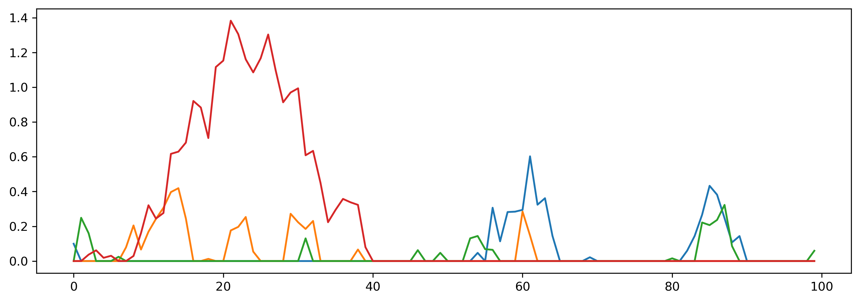
output_clocked represents the output of the neurons, which is a nnumpy array with shape (1, T, N). We can visualise this using matplotlib.
[6]:
plt.plot(output_clocked[0]);
Getting things done in time
Rockpool also offers a higher-level TimedModule interface, which accepts input and returns output as TimeSeries objects. TimeSeries objects provide a convenience encapsulation for handling time-series data, including both continuous signals and streams of events.
[7]:
# - Use the `.timed()` method to obtain a TimeSeries interface
tmod = mod.timed()
print(tmod)
TimedModuleWrapper  with shape (4, 4) {
    Rate '_module' with shape (4,)
} with Rate '_module' as module
timed() converts a low-level module into one which natively understands time series data. To test this out, we need to generate a time series!
Time series come in two flavours: TSContinuous for continous signals, and TSEvent for discrete event streams. In both cases they have their own internal time references, meaning the data can be sampled at arbitrary time points. See basics/time_series.ipynb for more information about TimeSeries objects.
[8]:
dt = 1e-3
T = 1000
time_base = np.arange(T) * dt

# - Generate a sinusoidal time series
freq = 2
ts_sin = TSContinuous(
    times=time_base,
    samples=np.sin(time_base * 2 * np.pi * freq),
    periodic=True,
    name="Sinusoid",
)
plt.figure()
ts_sin.plot()

# - Generate a noise time series
amp = 1
ts_noise = TSContinuous.from_clocked(
    samples=np.random.randn(T, N), dt=dt, periodic=True, name="White noise"
)
plt.figure()
ts_noise.plot();
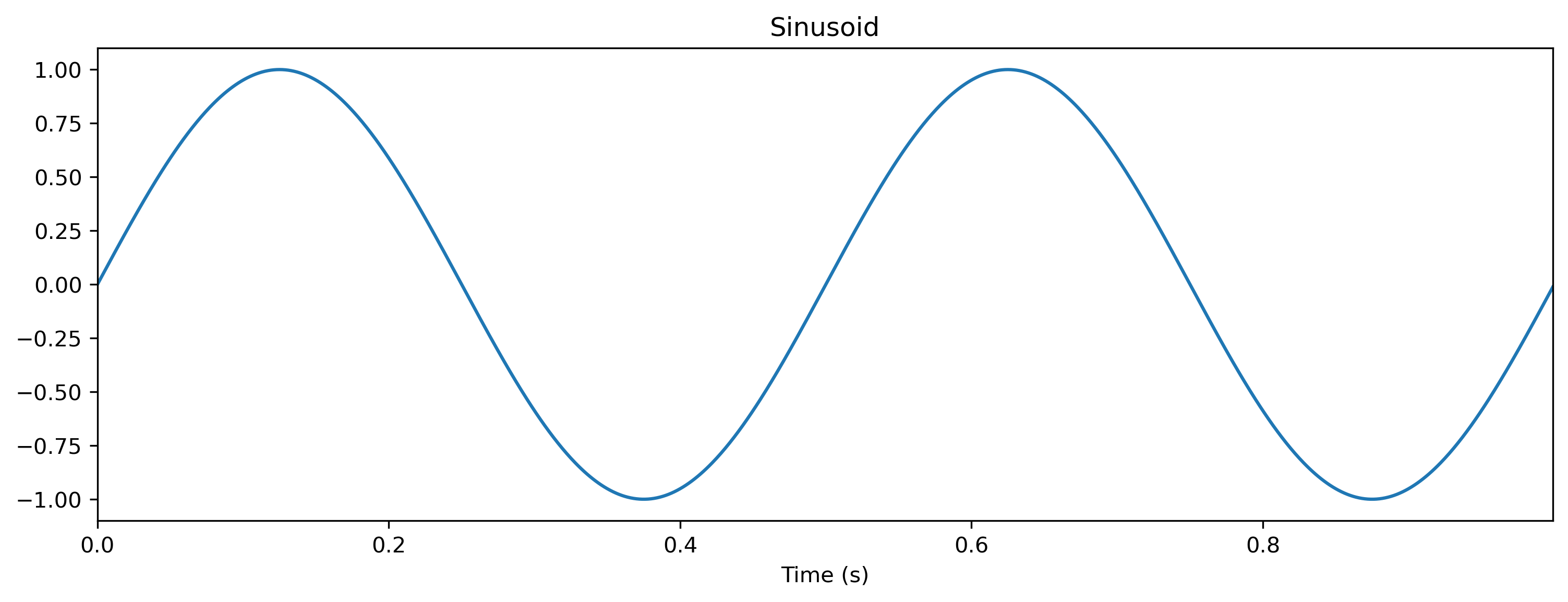
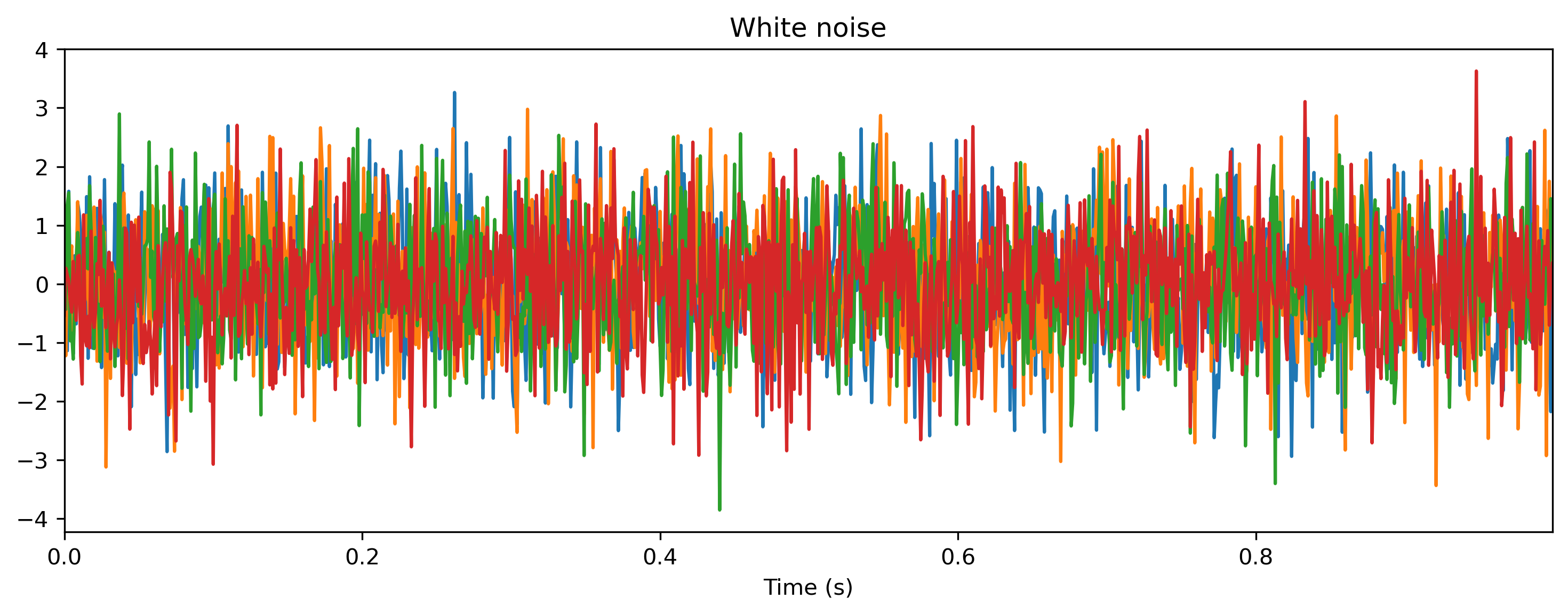
Here we used the TSContinous constructor to specify a time series with sample times times and values samples at the corresponding time points.
We used the TSContinusous.from_clocked() method to build a time series from regularly-sampled (“clocked”) data.
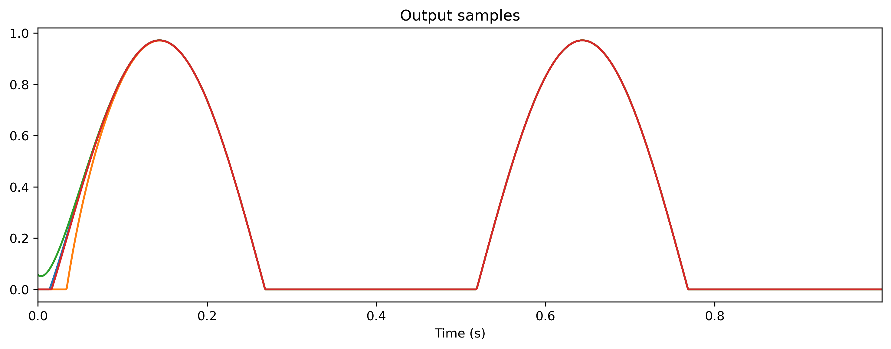
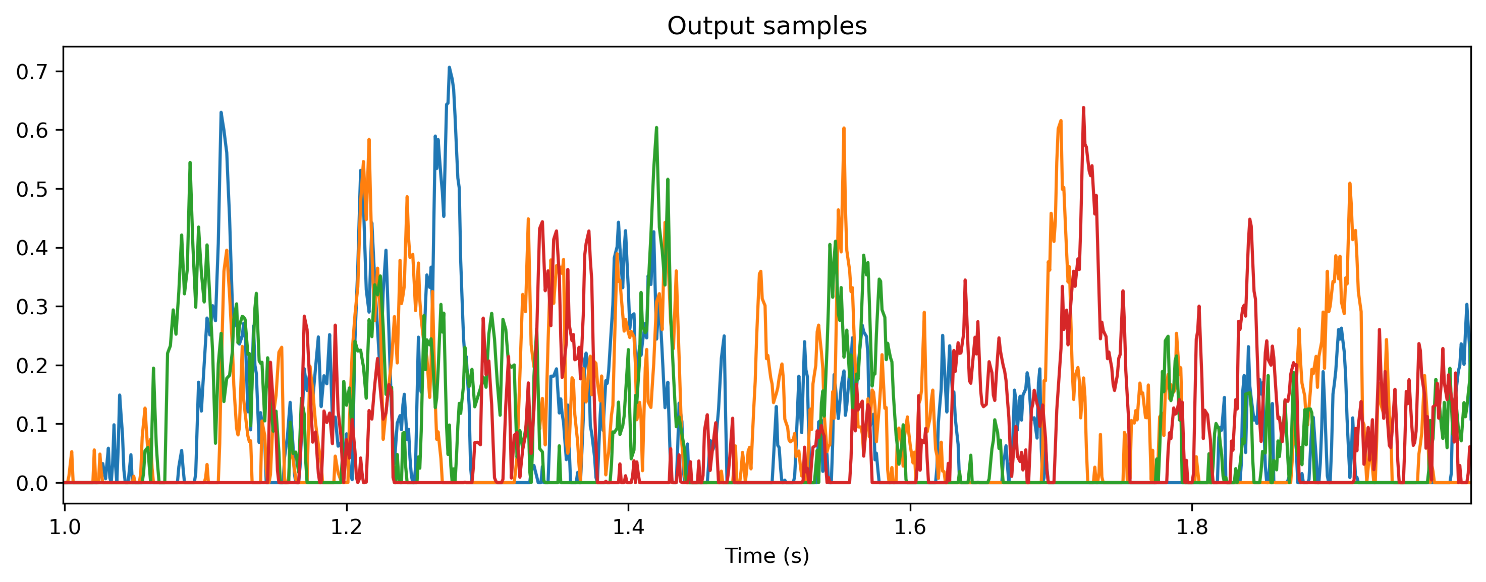
We can use time series such as these to push data through our TimedModule.
[9]:
# - Evolve the timed module
output, new_state, _ = tmod(ts_sin)
plt.figure()
output.plot()

output, new_state, _ = tmod(ts_noise)
plt.figure()
output.plot();
Building networks by composing and combining modules
Networks in Rockpool are also Module s that contain submodules, in a similar interface to PyTorch. This means you can easily build networks by composing and re-using submodules.
We provide a number of basic combinators to simply compose modules into more complex networks: for example Sequential and Residual. These combinators are all under the package rockpool.nn.combinators.
He we will define a very small feed-forward network, with one input channel, ten hidden units, and one output channel. This will require the modules Linear and Rate, and the combinator Sequential.
[10]:
# - Import the required modules
from rockpool.nn.modules import Linear, Rate

# - Import the `Sequential` combinator
from rockpool.nn.combinators import Sequential

# - Define the network size
input_size = 1
hidden_size = 10
output_size = 1

# - Build a sequential stack of modules
seqmod = Sequential(
    Linear((input_size, hidden_size)),
    Rate(hidden_size),
    Linear((hidden_size, input_size)),
)
print(seqmod)
ModSequential  with shape (1, 1) {
    Linear '0_Linear' with shape (1, 10)
    Rate '1_Rate' with shape (10,)
    Linear '2_Linear' with shape (10, 1)
}
We can once again call the module to pass data through the network.
[11]:
input_clocked = np.random.rand(T, 1)
output, state, _ = seqmod(input_clocked)
We can inspect the set of parameters and state of the module using the same methods as before, as well as the modules method to view submodules.
[12]:
print("Parameters:", seqmod.parameters(), "\n")
print("State:", seqmod.state(), "\n")
print("Modules:", seqmod.modules(), "\n")
Parameters:
{
    '0_Linear': {
        'weight': array([[ 1.00720834,  2.41430863,  2.05452097,  0.26908395,  0.87390412,
         0.16776011, -1.02723335, -2.21785861,  1.59488468,  1.98906917]])
    },
    '1_Rate': {
        'tau': array([0.02, 0.02, 0.02, 0.02, 0.02, 0.02, 0.02, 0.02, 0.02, 0.02]),
        'bias': array([0., 0., 0., 0., 0., 0., 0., 0., 0., 0.]),
        'threshold': array([0., 0., 0., 0., 0., 0., 0., 0., 0., 0.])
    },
    '2_Linear': {
        'weight': array([[-0.69257277],
       [-0.46641828],
       [-0.70623862],
       [ 0.57026507],
       [ 0.41529622],
       [-0.71813582],
       [ 0.20873922],
       [ 0.70115382],
       [-0.55436738],
       [-0.44933562]])
    }
}
State:
{
    '0_Linear': {},
    '1_Rate': {
        'x': array([ 0.45167469,  1.08267778,  0.92133383,  0.12066859,  0.39189545,
        0.07523071, -0.46065474, -0.99458131,  0.71521353,  0.89198248])
    },
    '2_Linear': {}
}
Modules:
OrderedDict([('0_Linear', Linear '0_Linear' with shape (1, 10)), ('1_Rate', Rate '1_Rate' with shape (10,)),
('2_Linear', Linear '2_Linear' with shape (10, 1))])
Parameters and states in Rockpool can be assigned families, such as “weights” and “taus”. This is used to to conveniently pull out classes of parameters, and can be passed as an argument to the parameters and state methods.
[13]:
print(seqmod.parameters("weights"))
{
    '0_Linear': {
        'weight': array([[ 1.00720834,  2.41430863,  2.05452097,  0.26908395,  0.87390412,
         0.16776011, -1.02723335, -2.21785861,  1.59488468,  1.98906917]])
    },
    '2_Linear': {
        'weight': array([[-0.69257277],
       [-0.46641828],
       [-0.70623862],
       [ 0.57026507],
       [ 0.41529622],
       [-0.71813582],
       [ 0.20873922],
       [ 0.70115382],
       [-0.55436738],
       [-0.44933562]])
    }
}
[14]:
# - Import the `OrderedDict` class
from collections import OrderedDict

# - Build an ordered dictionary of modules, specifying the name as each key
modules = OrderedDict([
    ("lin1", Linear((input_size, hidden_size))),
    ("rate1", Rate(hidden_size)),
    ("lin2", Linear((hidden_size, input_size))),
])

# - Build a `Sequential` network
seqmod = Sequential(modules)
print(seqmod)
ModSequential  with shape (1, 1) {
    Linear 'lin1' with shape (1, 10)
    Rate 'rate1' with shape (10,)
    Linear 'lin2' with shape (10, 1)
}
[15]:
# - Start with an empty `Sequential` network
seqmod = Sequential()

# - Append modules in turn, specifying the submodule names
seqmod.append(Linear((input_size, hidden_size)), "lin1")
seqmod.append(Rate(hidden_size), "rate1")
seqmod.append(Linear((hidden_size, input_size)), "lin2")

print(seqmod)
ModSequential  with shape (1, 1) {
    Linear 'lin1' with shape (1, 10)
    Rate 'rate1' with shape (10,)
    Linear 'lin2' with shape (10, 1)
}
Building a custom nested modules
You can build more complex custom network architectures by directly composing modules. Networks in Rockpool are all themselves Module subclasses. Here we’ll manually build a small reservoir network, with an input layer, a recurrent population, and an output layer of rate neurons.
We start by subclassing Module. We need to minimally define an __init__() method, which initialises the parameters and submodules of our network, and an evolve() method, which accepts input data, processes it and returns an output.
Important attributes in your module (e.g. parameters, state variables, etc.) should be wrapped with the Rockpool classes Parameter, State and SimulationParameter. This enables some of the convenience access methods of Rockpool, and is important for training. See the documentation for those classes for more information.
[16]:
# - Import the required modules
from rockpool.nn.modules import Linear, Rate, Module

# - Parameters are specified using the `Parameter` and `State`
from rockpool.parameters import Parameter, State, SimulationParameter

# - Design the network architecture
#   Every module inherits from Module
class net(Module):
    # - Every module needs an `__init__()` method to specify parameters
    def __init__(self, shape: tuple, *args, **kwargs):
        # - Every module must call `super().__init__()`
        super().__init__(shape, *args, **kwargs)

        # - Configure weight parameters
        self.w_input = Parameter(
            shape=self.shape[0:2],
            family="weights",
            init_func=lambda size: np.random.normal(size=size),
        )
        self.w_output = Parameter(
            shape=self.shape[1:],
            family="weights",
            init_func=lambda size: np.random.normal(size=size),
        )

        # - Build submodules
        self.mod_recurrent = Rate((shape[1], shape[1]), has_rec=True)

    # - Every module needs an `evolve()` method
    def evolve(self, input, record: bool = False) -> (np.array, np.array, dict):
        # - Initialise output arguments
        new_state = {}
        record_dict = {}

        # - Pass input through the input weights and submodule
        x, mod_state, mod_record_dict = self.mod_recurrent(
            np.dot(input, self.w_input), record
        )

        # - Maintain the submodule state and recorded state dictionaries
        new_state.update({"mod_recurrent": mod_state})
        record_dict.update({"mod_recurrent": mod_record_dict})

        # - Pass data through the output weights
        output = np.dot(x, self.w_output)

        # - Return outputs
        return output, new_state, record_dict
Now we can instantiate a module based on our net class, and test it by passing data through.
[17]:
# - Define the network size
input_size = 4
rec_size = 3
output_size = 2

# - Instantiate a module
net_mod = net(shape=(input_size, rec_size, output_size))
print(net_mod)
net  with shape (4, 3, 2) {
    Rate 'mod_recurrent' with shape (3, 3)
}
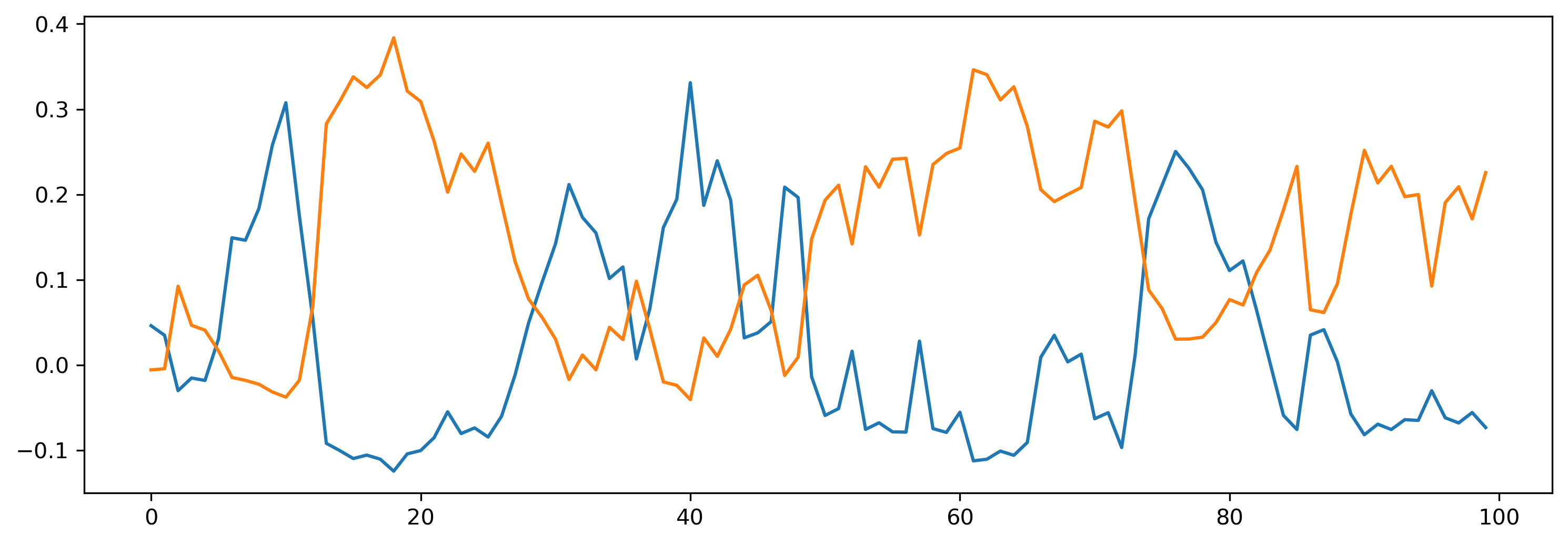
[18]:
# - Define an input
T = 100
input = np.random.randn(T, input_size)

# - Evolve the module
output, new_state, recorded_state = net_mod(input)
net_mod = net_mod.set_attributes(new_state)
plt.plot(output[0]);
If we inspect our network parameters, we can see they follow the structure of the module heirarchy, and include parameters defined by the sub-modules.
[19]:
print(net_mod.parameters())
{
    'w_input': array([[ 1.41978838, -1.13184915, -0.74752138],
       [-0.95091877,  0.30172439,  0.35265   ],
       [-0.09663117,  0.10782144, -1.36449476],
       [-0.72311345,  0.10093025, -0.2414413 ]]),
    'w_output': array([[-0.20141784,  0.62143563],
       [ 1.22627445, -0.14979523],
       [-1.53157303,  0.67460225]]),
    'mod_recurrent': {
        'w_rec': array([[ 0.15648791,  0.401766  , -1.14040351],
       [ 0.42543312,  0.5842613 , -0.30617398],
       [-0.81748013, -1.23444556, -0.26348427]]),
        'tau': array([0.02, 0.02, 0.02]),
        'bias': array([0., 0., 0.]),
        'threshold': array([0., 0., 0.])
    }
}
You can set the parameters of the network directly by setting attributes:
[20]:
# - Define weights
weights_in = np.random.rand(input_size, rec_size) - 0.5
weights_rec = np.random.randn(rec_size, rec_size) / rec_size
weights_out = np.random.rand(rec_size, output_size) - 0.5

# - Set the weights
net_mod.w_input = weights_in
net_mod.mod_recurrent.w_rec = weights_rec
net_mod.w_output = weights_out

# - Display the network
print(net_mod.parameters())
{
    'w_input': array([[ 0.28506196,  0.02794232,  0.05052549],
       [-0.39742499,  0.13996292, -0.191019  ],
       [-0.0180503 , -0.03285261,  0.01811005],
       [ 0.05156022, -0.23567097, -0.29003133]]),
    'w_output': array([[-0.28148003, -0.02212604],
       [-0.23931323,  0.24881792],
       [-0.41053964, -0.33932346]]),
    'mod_recurrent': {
        'w_rec': array([[-0.91369668,  0.15297224,  0.4534814 ],
       [ 0.05805358,  0.35401688, -0.29566064],
       [ 0.2393718 , -0.02951023, -0.00684574]]),
        'tau': array([0.02, 0.02, 0.02]),
        'bias': array([0., 0., 0.]),
        'threshold': array([0., 0., 0.])
    }
}
Next steps
Rockpool provides several additional niceties to make developing your own Module s easier. See the documentation for the Module class for more information.
You can also learn about Rockpool Parameter s, and about the facilities provided by the rockpool.utilities package.
See a simple example for training SNNs: 👋 Hello MNIST with Rockpool
Learn about the low-level API in detail: 🛠 Low-level Module API
Learn about the high-level API in detail: ⏱ High-level TimedModule API
Learn about the functional API in detail: [𝝺] Low-level functional API
Learn about training networks with Jax: 🏃🏽♀️ Training a Rockpool network with Jax
Lean about the Torch API: 🔥 Building Rockpool modules with Torch
Learn about training networks with Torch: 👩🏼🚒 Training a Rockpool network with Torch
Learn about training networks for deployment to hardware: 🐝 Overview of the Xylo™ family