This page was generated from docs/devices/xylo-imu/xylo-imu-intro.ipynb. Interactive online version:

🐝💨 Introduction to Xylo™IMU

XyloIMU is a platform for motion sensory processing, combining an IMU accelerometer sensor interface with a low-power SNN inference core. XyloIMU is designed for sub-mW motion processing, in always-on applications.

This notebook gives you an overview of interfacing from Rockpool to the various cores of Xylo-IMU.

See also 🐝⚡️ Quick-start with Xylo SNN core and ∿ The Xylo™IMU preprocessing interface.

# - General installation and imports
import sys
!{sys.executable} -m pip install --quiet matplotlib rich "rockpool[xylo, torch]"

# - Import numpy
import numpy as np

# - Configure matplotlib
import matplotlib.pyplot as plt
%matplotlib inline
plt.rcParams['figure.figsize'] = [12, 4]
plt.rcParams['figure.dpi'] = 300

# - Display images
from IPython.display import Image

import warnings
warnings.filterwarnings('ignore')

# - Nice printing
from rich import print

Overview of the Xylo™IMU design

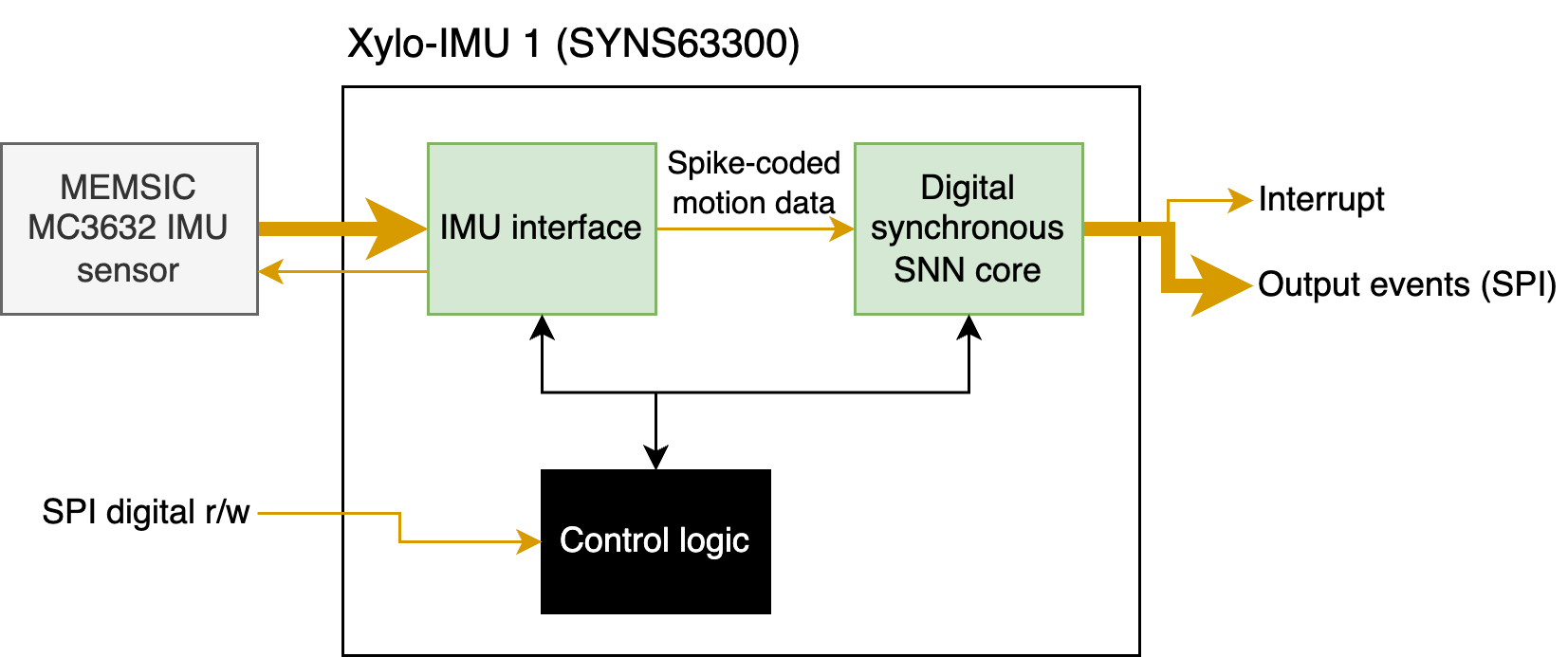
XyloIMU receives direct input from a MEMSIC MC3632 IMU sensor, and is designed to enable motion classification applications in real-time at low power.

The block-level outline of the chip is shown below. A dedicated IMU interface connects to the IMU sensor via a master SPI bus, and converts motion data into streams of events.

Event-encoded motion data is transferred to a digital SNN core for inference. The results of inference, encoded as output event streams, are transmitted over an interrupt bus or slave SPI bus to an external microcontroller.

A block of control logic manages configuration and communication with the cores. Configuration and readout from XyloIMU is performed over a slave SPI bus.

Image('xylo-imu-block-level.png')

Differences from other Xylo devices

XyloIMU is based around the same digital integer LIF inference core as the rest of the Xylo™ family. XyloIMU includes several design changes from XyloAudio 2 and other Xylo-family devices:

• One synaptic state per neuron

• 16 spiking input channels to SNN core

• 496 hidden neurons

• 16 spiking output channels

• Input weight projections to up to first 128 hidden neurons

• Output weight projection from up to 128 hidden neurons

• Up to 512 fanout recurrent weights per hidden neuron

• Up to 31,744 recurrent weights total

Part I: Using the SNN inference core on Xylo™IMU

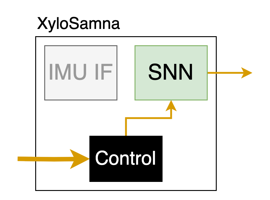
Interfacing with the Xylo SNN core is the same as for other Xylo family devices, making use of the Xylo deployment pipeline; XyloSim; and XyloSamna.

See also 🐝⚡️ Quick-start with Xylo SNN core and 🐝 Overview of the Xylo™ family.

Image('XyloSamna.png', width=400)

Step 1: Build a network in rockpool and convert it to a hardware configuration

# - Used to build trainable models
from rockpool.nn.modules import LIFTorch, LinearTorch
from rockpool.nn.combinators import Sequential, Residual

# - Modules required to interface and deploy models to the Xylo-IMU HDK
from rockpool.devices.xylo import find_xylo_hdks
from rockpool.devices.xylo.syns63300 import XyloSamna, config_from_specification, mapper, XyloSim
import rockpool.devices.xylo.syns63300.xylo_imu_devkit_utils as putils
from rockpool.transform import quantize_methods as q

# - Used for plotting time series
from rockpool import TSEvent, TSContinuous

# - Define the size of the network layers
Nin = 2
Nhidden = 4
Nout = 2
dt = 1e-2

# - Define the network architecture using combinators and modules
net = Sequential(
    LinearTorch((Nin, Nhidden), has_bias = False),
    LIFTorch(Nhidden, dt = dt),

    Residual(
        LinearTorch((Nhidden, Nhidden), has_bias = False),
        LIFTorch(Nhidden, has_rec = True, threshold = 1., dt = dt),
    ),

    LinearTorch((Nhidden, Nout), has_bias = False),
    LIFTorch(Nout, dt = dt),
)
print(net)

TorchSequential  with shape (2, 2) {
    LinearTorch '0_LinearTorch' with shape (2, 4)
    LIFTorch '1_LIFTorch' with shape (4, 4)
    TorchResidual '2_TorchResidual' with shape (4, 4) {
        LinearTorch '0_LinearTorch' with shape (4, 4)
        LIFTorch '1_LIFTorch' with shape (4, 4)
    }
    LinearTorch '3_LinearTorch' with shape (4, 2)
    LIFTorch '4_LIFTorch' with shape (2, 2)
}

# - Call the Xylo mapper on the extracted computational graph
spec = mapper(net.as_graph(),  weight_dtype='float', threshold_dtype='float', dash_dtype='float')

# - Quantize the specification
spec.update(q.global_quantize(**spec))

# # you can also try channel-wise quantization
# spec.update(q.channel_quantize(**spec))
# print(spec)

# - Use `config_from_specification()` to convert it to a hardware configuration
config, is_valid, msg = config_from_specification(**spec)
if not is_valid:
    print(msg)

Step 2: Deploy the network to the Xylo SNN core on a connected HDK

# - Find and connect to a Xylo IMU HDK
xylo_hdk_nodes, _, vers = find_xylo_hdks()
print(xylo_hdk_nodes, vers)

if len(xylo_hdk_nodes) == 0 or vers[0] != "syns63300":
    assert False, "This tutorial requires a connected Xylo IMU HDK to demonstrate."
else:
    db = xylo_hdk_nodes[0]

The connected Xylo HDK contains a Xylo IMU. Importing `rockpool.devices.xylo.syns63300`

[<samna.xyloImuBoards.XyloImuTestBoard object at 0x3508e55b0>]
['syns63300']

# - Use the `XyloSamna` module to deploy to the inference core on the HDK
modSamna = XyloSamna(db, config, dt = dt)
print(modSamna)

XyloSamna  with shape (2, 4, 2)

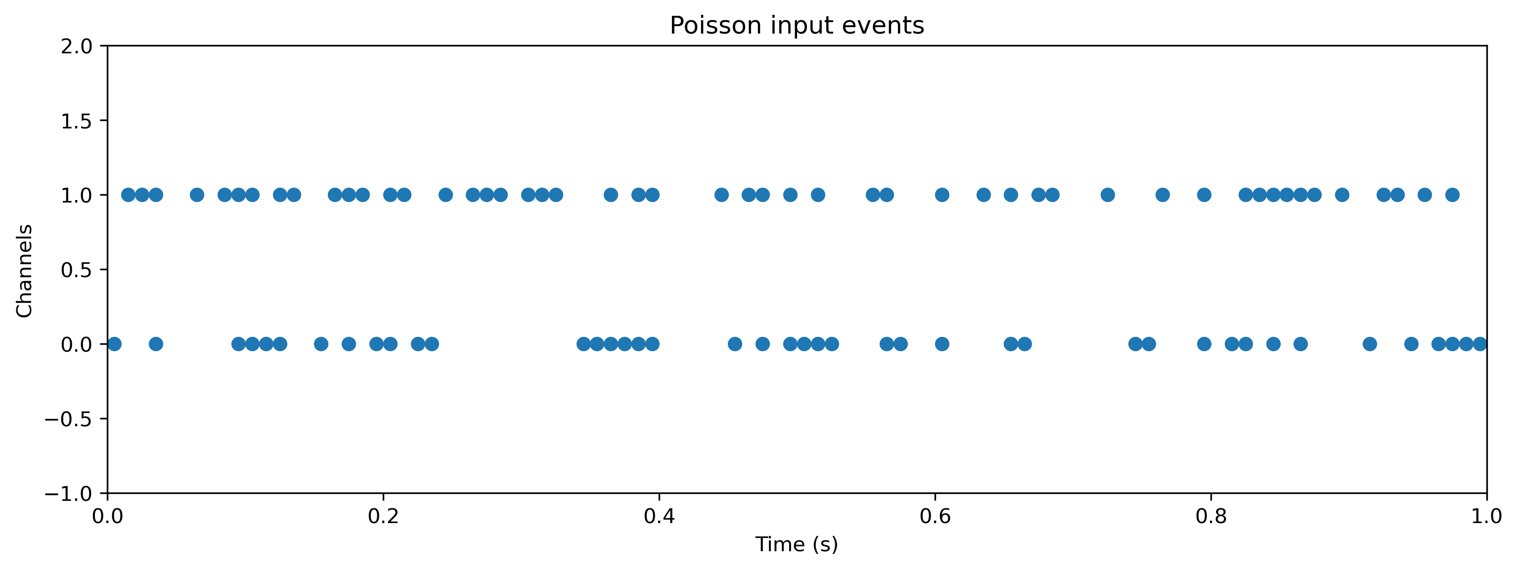
# - Generate some Poisson input
T = 100
f = 0.4
input_spikes = np.random.rand(T, Nin) < f
TSEvent.from_raster(input_spikes, dt, name = 'Poisson input events').plot();

# - Evolve the network on the Xylo HDK
out, _, r_d = modSamna.evolve(input_spikes.astype(int), record = True)

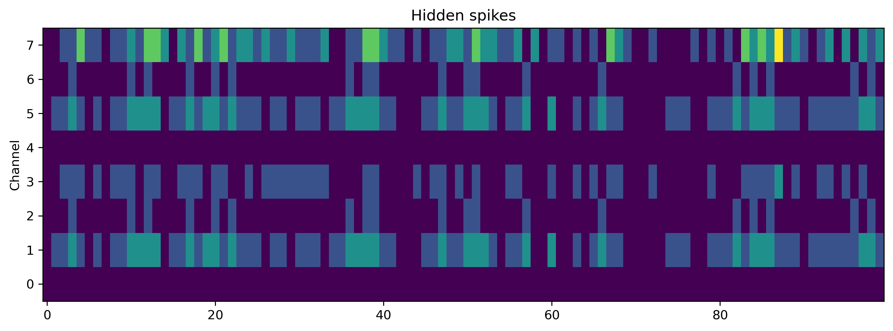
# - Show the internal state variables recorded
print(r_d.keys())

dict_keys(['Vmem', 'Isyn', 'Spikes', 'Vmem_out', 'Isyn_out', 'times'])

# - Plot some internal state variables
plt.figure()
plt.imshow(r_d['Spikes'].T, aspect = 'auto', origin = 'lower')
plt.title('Hidden spikes')
plt.ylabel('Channel')

plt.figure()
TSContinuous(r_d['times'], r_d['Vmem'], name = 'Hidden membrane potentials').plot(stagger = 127)

plt.figure()
TSContinuous(r_d['times'], r_d['Isyn'], name = 'Hidden synaptic currents').plot(stagger = 127);

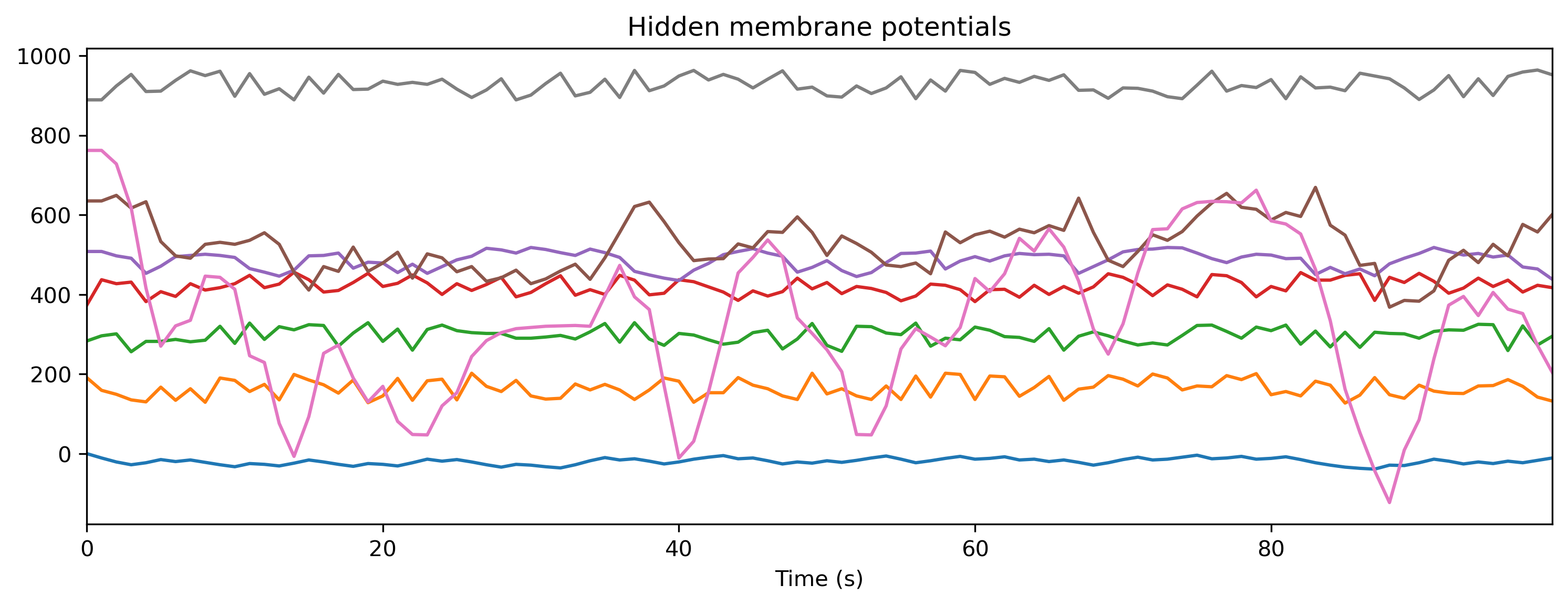
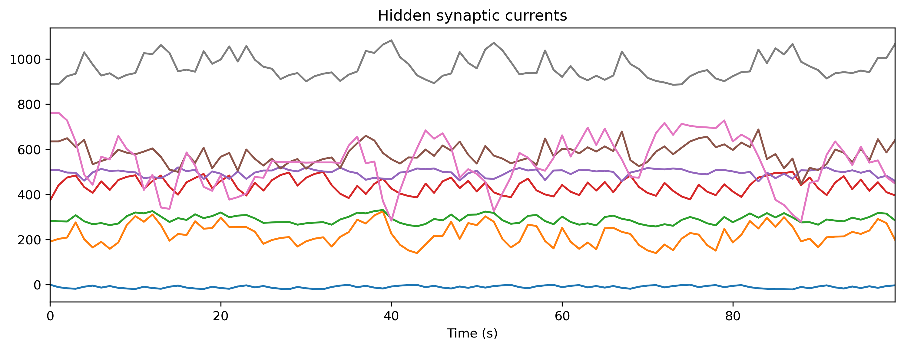
Step 3: Simulate the HDK using a bit-precise simulator

XyloSim is a bit-precise simulator of the Xylo SNN core. The version in the rockpool.devices.xylo.syns63300 package is tuned for Xylo IMU.

# - Use the XyloIMUSim device simulator
modSim = XyloSim.from_config(config, dt=dt)
print(modSim)

XyloSim  with shape (16, 1000, 8)

# - Evolve the input over the network, in simulation
out, _, r_d = modSim(input_spikes, record = True)

# - Show the internal state variables recorded
print(r_d.keys())

dict_keys(['Vmem', 'Isyn', 'Spikes', 'Vmem_out', 'Isyn_out'])

# - Plot some internal state variables
plt.figure()
plt.imshow(r_d['Spikes'].T, aspect = 'auto', origin = 'lower')
plt.title('Hidden spikes')
plt.ylabel('Channel')

plt.figure()
TSContinuous.from_clocked(r_d['Vmem'], dt, name = 'Hidden membrane potentials').plot(stagger = 127)

plt.figure()
TSContinuous.from_clocked(r_d['Isyn'], dt, name = 'Hidden synaptic currents').plot(stagger = 127);

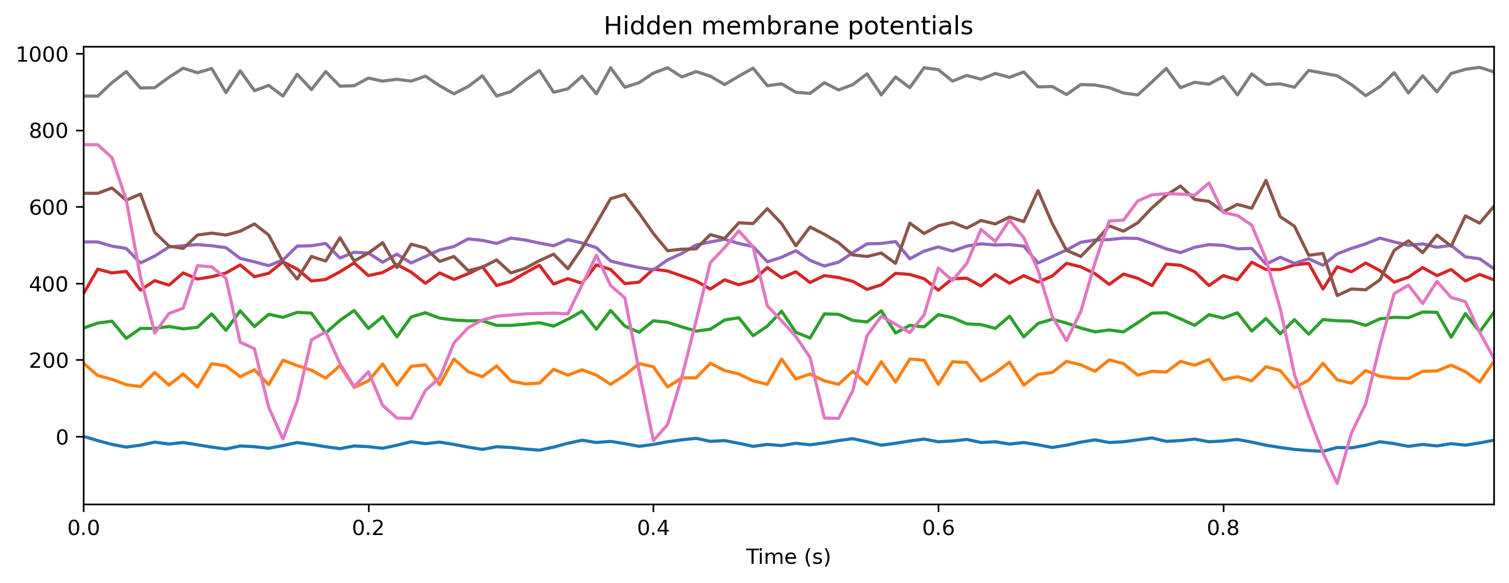
PART II: The IMU encoding interface

XyloIMU incorporates an efficient event encoding block for IMU motion data, which includes removal / correction of rotation by detection the gravity-associated force vector.

For a more detailed description of the interface, see ∿ The Xylo™IMU preprocessing interface.

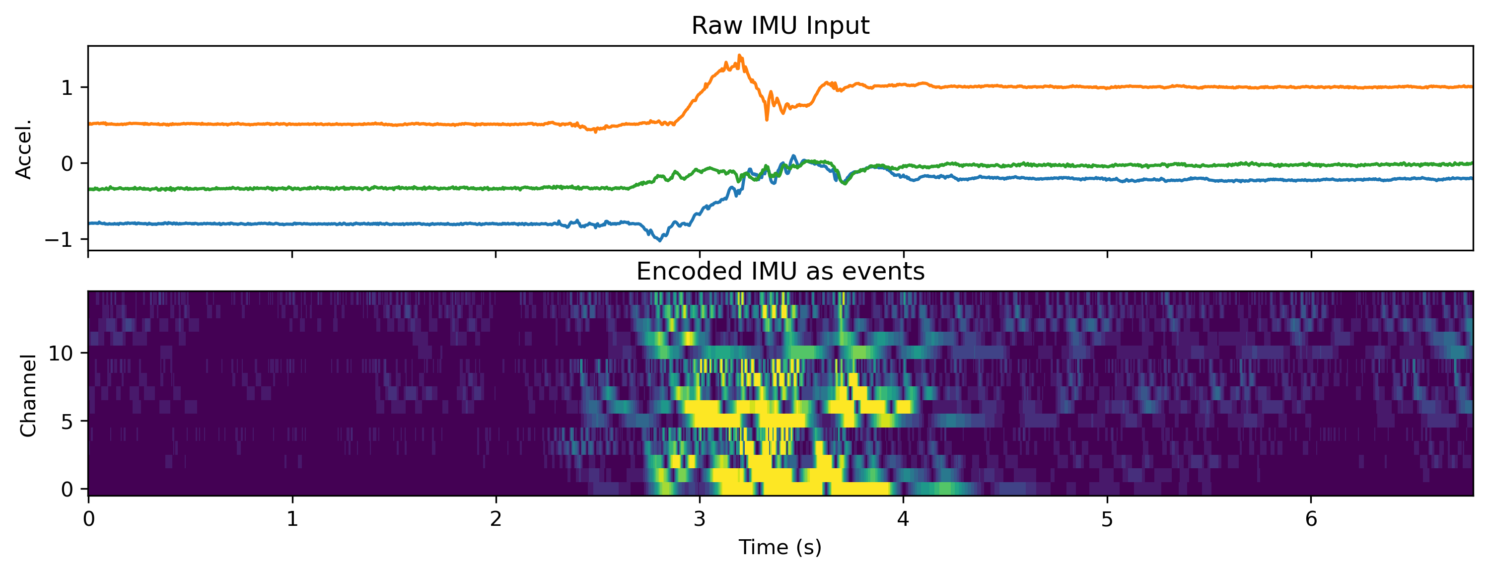
The block diagram below shows the main steps in preprocessing IMU data to events. Three channels of IMU input (x, y, z) are converted to 15 event channels (5 per sensor channel), which are then sent to the Xylo SNN inference core.

Rockpool includes a bit-accurate simulation of the IMU conversion interface, in IMUIFSim.

This simulator allows you to encode IMU motion data as events in the same way as live IMU data on Xylo-IMU, for use in training and testing applications.

Image('IMU-IF-block-level.png')

Using the IMU IF Simulation module

See also ∿ The Xylo™IMU preprocessing interface and 🧑‍🏫 Specifying IMU preprocessing parameters

from rockpool.devices.xylo.syns63300 import IMUIFSim

# - Load a dummy IMU sample
input_data = np.load('data.npy')

# - Create an IMUIFSim module
mod = IMUIFSim()
print(mod)

IMUIFSim  with shape (3, 15) {
    ModSequential 'model' with shape (3, 15) {
        RotationRemoval '0_RotationRemoval' with shape (3, 3) {
            ModSequential 'sub_estimate' with shape (3, 9) {
                SubSpace '0_SubSpace' with shape (3, 9)
                SampleAndHold '1_SampleAndHold' with shape (9, 9)
            }
        }
        FilterBank '1_FilterBank' with shape (3, 15)
        ScaleSpikeEncoder '2_ScaleSpikeEncoder' with shape (15, 15)
    }
}

IMUIFSim is a standard Rockpool module accepting raw IMU data, and returning encoded events.

# - Quantize the raw IMU data
from rockpool.devices.xylo.syns63300 import Quantizer
quantizer = Quantizer(shape=3, scale=0.49, num_bits=16)
Q_data, _, _ = quantizer(input_data)

# - Test evolution and plot input and output
out, _, r_d = mod(Q_data, record = True)

times = np.arange(0, input_data.shape[0]) * mod.dt
ax = plt.subplot(2, 1, 1)
ax.plot(times, input_data)
ax.set_xlim(0, times[-1])
ax.set_xticklabels([])
ax.set_title('Raw IMU Input')
ax.set_ylabel('Accel.')

ax = plt.subplot(2, 1, 2)
ax.imshow(out[0].astype(int).T, aspect='auto', interpolation='none', origin='lower')
ax.set_xticklabels(np.array(ax.get_xticks() * mod.dt).astype(int))
ax.set_title('Encoded IMU as events')
ax.set_xlabel('Time (s)')
ax.set_ylabel('Channel');

Using the export_config() method, you can obtain a hardware configuration object with which you can configure the encoding block on Xylo IMU.

if_config = mod.export_config()
print(if_config)

xyloImu::configuration::InputInterfaceConfig(enable=1, configuration_timeout=3.000000, estimator_k_setting=4,
select_iaf_output=0, bypass_jsvd=0, update_matrix_threshold=10, delay_threshold=500, bpf_bb_values={ 6 5 4 3 2 6 5
4 3 2 6 5 4 3 2 }, bpf_bwf_values={ 8 8 8 8 8 8 8 8 8 8 8 8 8 8 8 }, bpf_baf_values={ 9 10 11 12 13 9 10 11 12 13 9
10 11 12 13 }, bpf_a1_values={ -64458 -63288 -60684 -54529 -39246 -64458 -63288 -60684 -54529 -39246 -64458 -63288
-60684 -54529 -39246 }, bpf_a2_values={ 31754 30771 28888 25417 19378 31754 30771 28888 25417 19378 31754 30771
28888 25417 19378 }, scale_values={ 5 5 5 5 5 5 5 5 5 5 5 5 5 5 5 }, iaf_threshold_values={ 1024 1024 1024 1024
1024 1024 1024 1024 1024 1024 1024 1024 1024 1024 1024 })

IMUIFSim supports all optional features of the IMU encoding interface. See 🧑‍🏫 Specifying IMU preprocessing parameters for more detail on how to specify the parameters of the IMU IF.

Accessing the IMU encoding interface on HW

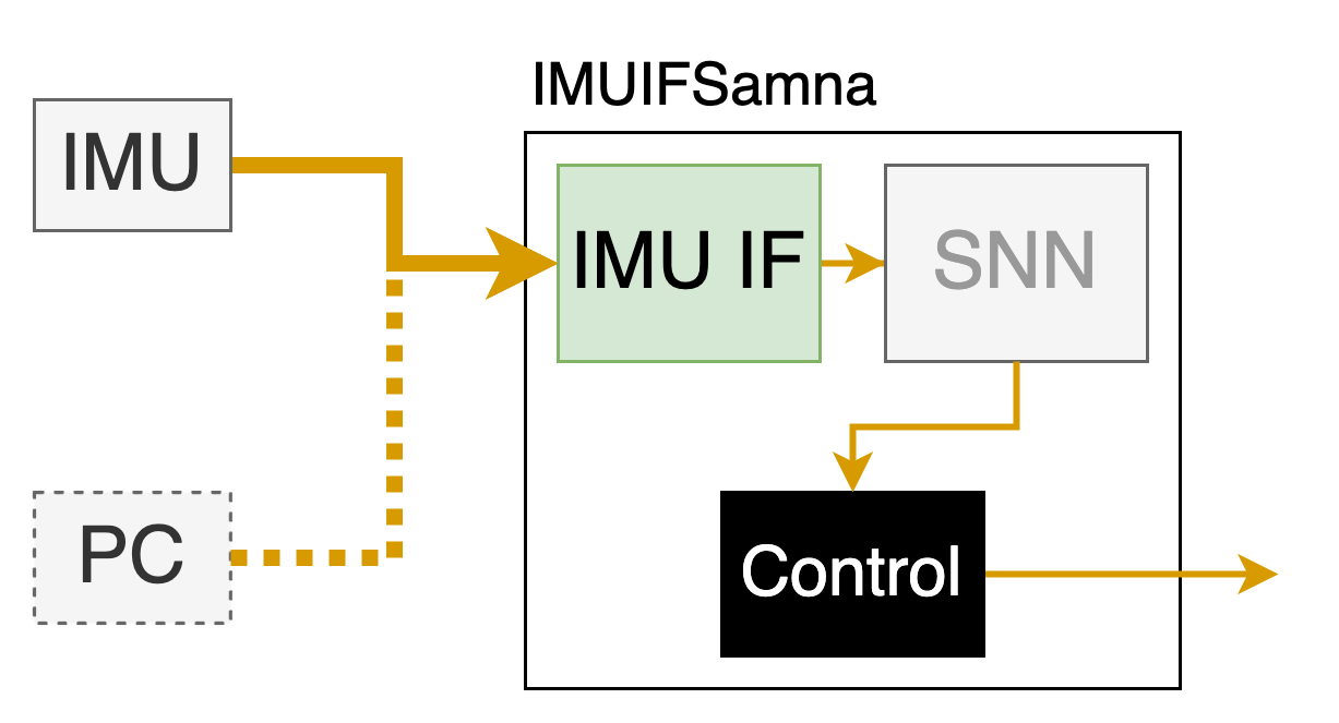
Rockpool also provides a module IMUIFSamna to record encoded data from the IMU interface on XyloIMU. The IMU sensor data can come either from the on-board IMU chip, or from pre-recorded data streamed from the host PC.

Warning

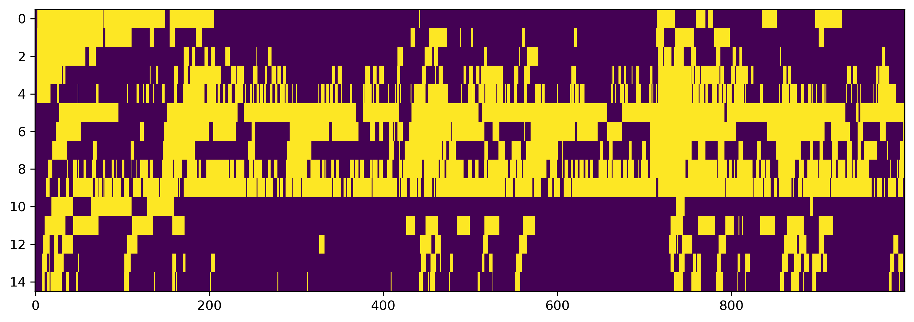
IMUIFSamna currently uses a work-around to record encoded IMU data as events. It is only capable of recording one event per time-step per channel from the IMU interface. However, the IMU interface is capable of producing multiple events per time-step per channel. As a result, data recorded using IMUIFSamna may differ from that transmitted to the SNN core on Xylo IMU. You can alternatively use IMUData to record raw IMU data, and IMUIFSim to encode that data, supporting multiple events per time-step per channel. This may result in more accurate encoding of data.

Image('IMUIFSamna.png', width=400)

# - Import the required Rockpool module
from rockpool.devices.xylo.syns63300 import IMUIFSamna

# - Instantiate the module, connected to an HDK `db`
imu_if = IMUIFSamna(db, prerecorded_imu_input = False)

# - You can also supply pre-recorded IMU data, and specify the IMU IF parameters
# IMUIFSamna(db, prerecorded_imu_input = True, interface_params={})

# - Record for 1000 time steps, by providing zero data
out, _, _ = imu_if(np.zeros((1000, 3)))

# times, channels = np.where(out)
# plt.scatter(times, channels)

plt.imshow(out.T, aspect = 'auto', interpolation = 'none')

<matplotlib.image.AxesImage at 0x386214310>

Delete the module to release access to the IMU sensor.

del imu_if

[2024-06-07 13:03:24.926] [Graph] [warning] Graph is destroyed while running! Note: Filter nodes constructed by `sequential` method won't work after corresponding graph is destroyed and please manually stop the graph after use.

PART III: Recording live IMU data

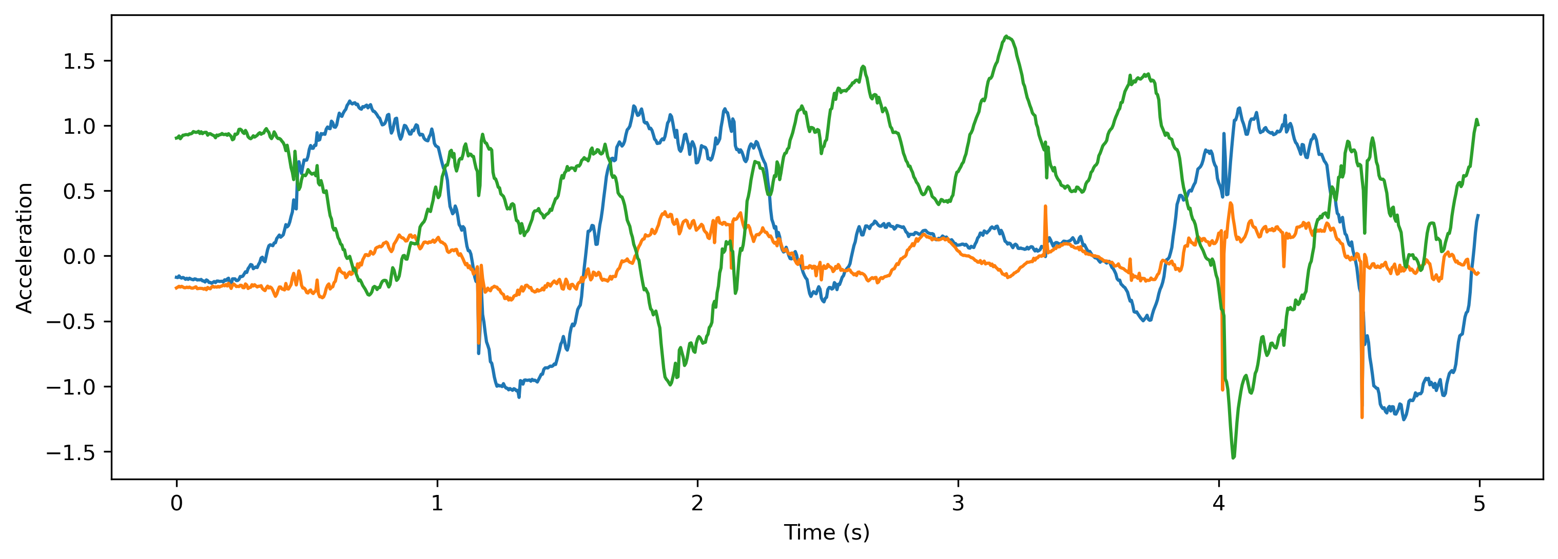
Rockpool provides a module IMUData to record raw IMU data from the MEMSIC IMU Sensor on the XyloIMU HDK. This can be used to record live IMU input, or to record IMU data to build a training dataset.

Image('IMUData.png', width=400)

# - Import and instantiate and IMUData module
from rockpool.devices.xylo.syns63300 import IMUData

mod = IMUData(db)
print(mod)

IMUData  with shape (0, 3)

IMUData is a standard Rockpool module, which returns real-time samples recorded from the IMU device on a Xylo IMU HDK. Use a zero-element numpy array to specify how many samples to record.

dt = mod.dt # By default Xylo IMU operates at 200 Hz
T = int(5. / dt) # Record for 5 seconds

# - Record live IMU sensor data
data, _, _ = mod(np.zeros((0, T, 0)))

# - Plot the data samples
times = np.arange(0, T) * mod.dt
plt.plot(times, data)
plt.xlabel('Time (s)')
plt.ylabel('Acceleration');

PART IV: Real-time streaming mode

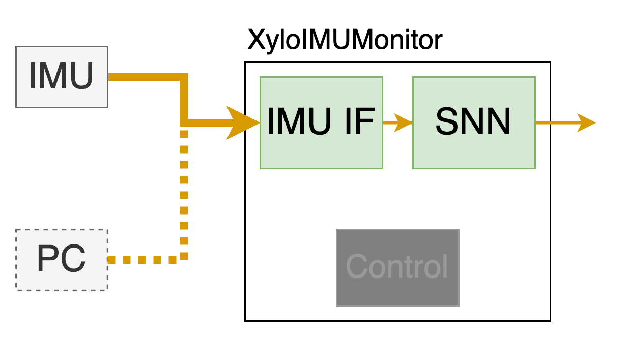
The streaming mode combines the IMU interface and SNN inference core modules together in real time using the class XyloIMUMonitor. In this mode you only read the output events from the SNN core, with input either from the live IMU sensor, or streamed from a PC.

Image('XyloIMUMonitor.png', width = 400)

Step 1: Build a network in rockpool and convert it to a hardware configuration

# - Define the size of the network layers
Nin = 15
Nhidden = 4
Nout = 2
dt = 1. / 200

# - Define the network architecture using combinators and modules
net = Sequential(
    LinearTorch((Nin, Nhidden), has_bias = False),
    LIFTorch(Nhidden, dt = dt),

    Residual(
        LinearTorch((Nhidden, Nhidden), has_bias = False),
        LIFTorch(Nhidden, has_rec = True, threshold = 1., dt = dt),
    ),

    LinearTorch((Nhidden, Nout), has_bias = False),
    LIFTorch(Nout, dt = dt),
)
print(net)

TorchSequential  with shape (15, 2) {
    LinearTorch '0_LinearTorch' with shape (15, 4)
    LIFTorch '1_LIFTorch' with shape (4, 4)
    TorchResidual '2_TorchResidual' with shape (4, 4) {
        LinearTorch '0_LinearTorch' with shape (4, 4)
        LIFTorch '1_LIFTorch' with shape (4, 4)
    }
    LinearTorch '3_LinearTorch' with shape (4, 2)
    LIFTorch '4_LIFTorch' with shape (2, 2)
}

# - Call the Xylo mapper on the extracted computational graph
spec = mapper(net.as_graph(),  weight_dtype='float', threshold_dtype='float', dash_dtype='float')

# - Quantize the specification
spec.update(q.global_quantize(**spec))

# # you can also try channel-wise quantization
# spec.update(q.channel_quantize(**spec))
# print(spec)

# - Use rockpool.devices.xylo.config_from_specification to convert it to a hardware configuration
config, is_valid, msg = config_from_specification(**spec)
if not is_valid:
    print(msg)

Step 2: Deploy the network on chip and run simulation

# - Find and connect to a Xylo IMU HDK
xylo_hdk_nodes, _, vers = find_xylo_hdks()
print(xylo_hdk_nodes, vers)

if len(xylo_hdk_nodes) == 0 or vers[0] != 'syns63300':
    assert False, 'This tutorial requires a connected Xylo IMU HDK to demonstrate.'
else:
    db = xylo_hdk_nodes[0]

The connected Xylo HDK contains a Xylo IMU. Importing `rockpool.devices.xylo.syns63300`

[<samna.xyloImuBoards.XyloImuTestBoard object at 0x3508e55b0>]
['syns63300']

# - Use the `XyloIMUMonitor` module to deploy to the HDK, running in real time
from rockpool.devices.xylo.syns63300 import XyloIMUMonitor

output_mode = "Vmem"

modMonitor = XyloIMUMonitor(device=db, config=config, dt=dt, output_mode=output_mode)

# - A resultList stack to store the results
from IPython.display import clear_output

class ResultList(object):
    def __init__(self, max_len=100):
        self._list = []
        self.max_len = max_len

    def reset(self):
        self._list = []

    def append(self, num):
        if len(self._list) < self.max_len:
            self._list.append(num)
        else:
            self._list[: self.max_len - 1] = self._list[1:]
            self._list[self.max_len - 1] = num

    def is_full(self):
        if len(self._list) == self.max_len:
            return True
        else:
            return False

    def counts(self, features=[]):
        count = 0
        for _ in self._list:
            if _ in features:
                count += 1
        return count

    def __len__(self):
        return len(self._list)

    @property
    def list(self):
        return self._list

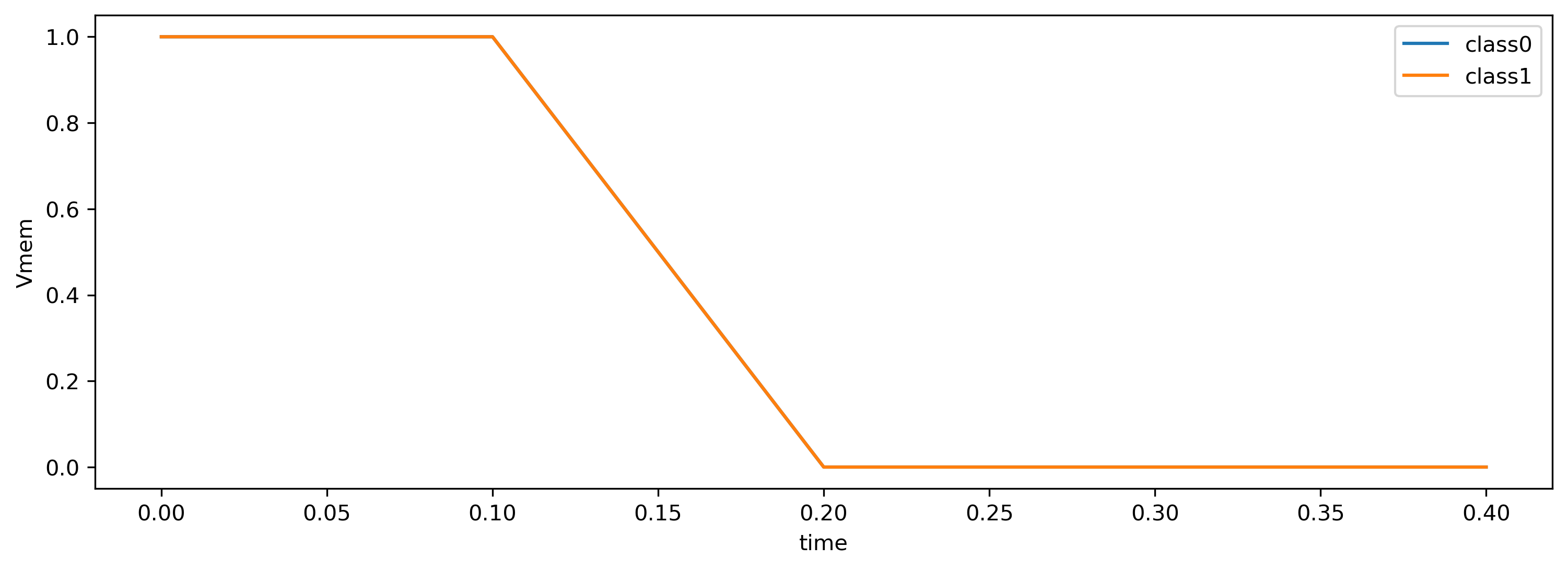
# - Draw a real time image for output channels, you can shake the Xylo IMU device while running

lines = [ResultList(max_len=10) for _ in range(Nout)]
time_base = ResultList(max_len=10)
tt = 0
T = 200
t_inference = 10.

from time import time

t_start = time()

while (time() - t_start) < t_inference:
    # - Perform inference on the Xylo IMU HDK
    output, _, _ = modMonitor(input_data=np.zeros((T, 3)))
    if output is not None:
        output = np.max(output, axis=0)
        for i in range(Nout):
            lines[i].append(output[i])

        time_base.append(tt)
        tt += 0.1
        ax_time = time_base.list

        for i in range(Nout):
            plt.plot(ax_time, lines[i].list, label=f"class{i}")

        plt.xlabel('time')
        plt.ylabel('Vmem')
        plt.legend()
        plt.pause(0.1)
        clear_output(wait=True)

Part V: Measuring power on the Xylo HDK

XyloSamna provides an interface to real-time power measurements on the Xylo™IMU HDK. Current on several power nets on the chip can be sampled asynchronously, while the device is in operation.

The evolve() method provides a power measurement interface while the device is in inference mode, and the XyloSamna module can be used also to measure idle power.

# - Find and connect to a Xylo IMU HDK
xylo_hdk_nodes, modules, versions = find_xylo_hdks()
print(xylo_hdk_nodes, versions)

if len(xylo_hdk_nodes) == 0 or versions[0] is not 'syns63300':
    assert False, 'This tutorial requires a connected Xylo IMU HDK to demonstrate.'
else:
    db = xylo_hdk_nodes[0]
    x = modules[0]

The connected Xylo HDK contains a Xylo IMU. Importing `rockpool.devices.xylo.syns63300`

[<samna.xyloImuBoards.XyloImuTestBoard object at 0x3508e55b0>]
['syns63300']

On instantiation, XyloSamna can specify a power sampling frequency. By default, power is measured at 5 Hz. Below we increase this to 20 Hz.

# - Set a low clock frequency for the Xylo device
print(f'Setting Xylo main clock to {x.xylo_imu_devkit_utils.set_xylo_core_clock_freq(db, 6.25)} MHz')

# - Use XyloSamna to deploy to the HDK
modSamna = x.XyloSamna(db, config, dt = 10e-3, power_frequency=20.)
print(modSamna)

Setting Xylo main clock to 6.25 MHz

XyloSamna  with shape (15, 4, 2)

# - Generate some Poisson input
T = 1000
f = 0.4
input_spikes = np.random.rand(T, Nin) < f

# - Evolve some input on the SNN core, and record power during inference
out, _, record_dict = modSamna(input_spikes, record_power = True)

print(record_dict)

{
    'io_power': array([0.0003336 , 0.00032705, 0.00033385, 0.00033586, 0.00033284,
       0.00033083, 0.00032629, 0.00034039]),
    'core_power': array([0.00019518, 0.00020046, 0.00021628, 0.00018991, 0.00019518,
       0.00021101, 0.00020046, 0.00020046])
}

Power is sampled on two nets, and is returned in Watts.

'io_power' is the total I/O power of the device. 'core_power' is the power consumption of the digital SNN core and control logic.

print(f"Active IO power:\t{np.mean(record_dict['io_power']) * 1e6}µW\nSNN + IMU IF core:\t{np.mean(record_dict['core_power']) * 1e6}µW")

Active IO power:        332.58819580078125µW
SNN + IMU IF core:      201.11628941127233µW

# - Measure idle power (no evolution)
from time import sleep

modSamna._power_buf.clear_events()
sleep(5.)
power = modSamna._power_buf.get_events()

power_idle = ([], [])

for p in power:
    power_idle[p.channel].append(p.value)

idle_power_per_channel = np.mean(np.stack(power_idle), axis = 1)

print(f'Idle IO power:\t\t{idle_power_per_channel[0] * 1e6}µW\nSNN + IMU IF core:\t{idle_power_per_channel[1]*1e6}µW')

Idle IO power:          334.30778503417963µW
SNN + IMU IF core:      188.16571916852678µW

Hints on reducing power consumption

Several points may be useful in reducing active power on XyloIMU.

• Reducing the core clock frequency. The dev-kit utility function devices.xylo.imu.xylo_imu_devkit_utils.set_xylo_core_clock_freq() can be used to set a lower core clock frequency than the default of 50 Mhz, lowering power consumption proportionally. Depending on your network size and complexity you can most likely reduce the clock frequency and still guarantee real-time operation.

• Reducing network activity and network size. The SNN core within Xylo only works as hard as it needs to. Once all neuron states have been updated, the core performs no operations until the next network time-step. This conserves energy.

help(x.xylo_imu_devkit_utils.set_xylo_core_clock_freq)

Help on function set_xylo_core_clock_freq in module rockpool.devices.xylo.syns63300.xylo_imu_devkit_utils:

set_xylo_core_clock_freq(device: samna.xyloImuBoards.XyloImuTestBoard, desired_freq_MHz: float) -> float
    Set the inference core clock frequency used by Xylo

    Args:
        device (XyloIMUHDK): A Xylo device to configure
        desired_freq_MHz (float): The desired Xylo core clock frequency in MHz

    Returns:
        (float): Actual frequency obtained, in MHz

Estimate the required master clock frequency for real-time operation

Rockpool includes a model of the cycles required to operate the Xylo SNN inference core, in cycles_model(). Xylo is an efficient device, which skips computation whenever possible. As a result, the computational requirements and power consumption vary dynamically with network activity, and with network configuration.

By default cycles_model() estimates a worst-case scenario, which can inform the master clock frequency that guarantees real-time operation for your network. It can also take into account real network activity to estimate a usual computational load.

The function est_clock_freq() will return the master clock frequency that guarantees real-time operation, for a given Xylo configuration.

from rockpool.devices.xylo.syns63300 import cycles_model, est_clock_freq

help(cycles_model)

Help on function cycles_model in module rockpool.devices.xylo.syns63300.power_cycles_model:

cycles_model(config: samna.xyloImu.configuration.XyloConfiguration, input_sp: Union[float, numpy.ndarray, torch.Tensor, array] = 1.0, hidden_sp: Union[float, numpy.ndarray, torch.Tensor, array] = 1.0, output_sp: Union[float, numpy.ndarray, torch.Tensor, array] = 1.0) -> float
    Calculate the average number of cycles required for a given network architecture

    This function contains a model which estimates the number of master clock cycles required for the Xylo SNN SYNS61202 inference core to compute one time-step for a given chip configuration in ``config``. Use :py:func:`.devices.xylo.syns61201.config_from_specification` to obtain a chip configuration, along with :py:meth:`.Module.as_graph` and :py:func:`.devices.xylo.syns61201.mapper`, as described in the deployment tutorials for Xylo.

    By default the model provides a "worst-case" estimation, assuming that every neuron and every input channel fire on each time-step. If desired, real input rasters and real hidden and output spike rasters can be provided for analysis. Alternative spiking probabilities can also be provided as floats ``0..1``.

    Note that when estimating spiking probablility, only boolean values are relevant --- either a spike or no spike per time step per channel. Multiple events per bin cost the same as a single event.

    Args:
        config (XyloIMUConfig): A Xylo IMU configuration for which to calculate the cycle requirements
        input_sp (FloatVector): Either a floating-point number 0..1, specifying the average input firing rate, or an actual input spike raster to use in evaluation. Default: `1.0`; estimate a worst-case scenario
        hidden_sp (FloatVector): Either a floating-point number 0..1, specifying the average hidden neuron firing rate, or an actual hidden spike raster to use in evaluation. Default: `1.0`; estimate a worst-case scenario
        output_sp (FloatVector): Either a floating-point number 0..1, specifying the average output neuron firing rate, or an actual output spike raster to use in evaluation. Default: `1.0`; estimate a worst-case scenario

    Returns:
        float: The average number of master clock cycles required for this configuration, for the Xylo SNN core to compute one network `dt`

help(est_clock_freq)

Help on function est_clock_freq in module rockpool.devices.xylo.syns63300.power_cycles_model:

est_clock_freq(config: samna.xyloImu.configuration.XyloConfiguration, dt: float, margin: float = 0.2)
    Estimate the required master clock frequency, to run a network in real-time

    This function will perform a worst-case analysis, assuming that every input channel, every hidden neuron and every output neuron fire an event on each `dt`. An additional margin is included (Default: 20%), to guarantee that the model will run in real time at the suggested master clock frequency.

    Args:
        config (XyloIMUConfig):  A Xylo IMU configuration for which to estimate the required clock frequency
        dt (float): The required network `dt`, in seconds
        margin (float): The additional overhead safety margin to add to the estimation, as a fraction. Default: `0.2` (20%)

print(f"This network requires {cycles_model(config)} master clock cycles per network time-step.")
print(f"This network requires a master clock of {est_clock_freq(config, dt) / 1e6:.2f} MHz for real-time operation.")

This network requires 757.0 master clock cycles per network time-step.

This network requires a master clock of 0.18 MHz for real-time operation.

Next steps

See ∿ The Xylo™IMU preprocessing interface for more detail about the IMU encoding interface.

See 🧑‍🏫 Specifying IMU preprocessing parameters for details of how to configure the preprocessing and encoding modules.