This page was generated from docs/devices/quick-xylo/deploy_to_xylo.ipynb. Interactive online version:

🐝⚡️ Quick-start with Xylo SNN core

This notebook gives you an ultra-quick overview of taking a network from high-level Python simulation through to deployment to HDKs with Xylo SNN cores.

The notebook shows you

• how to build a network with Rockpool, using standard network modules and combinators

• how to extract the computational graph for that network, containing all parameters needed to specify the network on a Xylo HDK

• how to map the computational graph to the Xylo HW, assigning hardware resources for the network

• how to quantize the network specification to match the integer SNN core on Xylo, and obtain a hardware configuration

• how to connect to and configure the Xylo HDK hardware, to deploy the network

• how to evaluate the network on the Xylo HDK

• how to simulate the configuration in a bit-precise simulator of the Xylo HDK.

# - Numpy
import numpy as np

# - Matplotlib
import sys
!{sys.executable} -m pip install --quiet matplotlib
import matplotlib.pyplot as plt
%matplotlib inline
plt.rcParams['figure.figsize'] = [12, 4]
plt.rcParams['figure.dpi'] = 300

# - Rockpool time-series handling
from rockpool import TSEvent, TSContinuous

# - Pretty printing
try:
    from rich import print
except:
    pass

# - Display images
from IPython.display import Image

# - Disable warnings
import warnings
warnings.filterwarnings('ignore')

Xylo in numbers

These are the most important numbers to keep in mind when building networks for Xylo. See also 🐝 Overview of the Xylo family. Note that the network size constraints apply only to the Xylo hardware via XyloSamna, and you can simulate larger networks using XyloSim.

Description	Number
Max. input channels	16
Max. input spikes per time step	15
Max. hidden neurons	1000
Max. hidden neuron spikes per time step	31
Max. input synapses per hidden neuron	2
Max. alias targets (hidden neurons only)	1
Max. output neurons	8
Max. output neuron spikes per time step	1
Max. input synapses per output neuron	1
Weight bit-depth	8
Synaptic state bit-depth	16
Membrane state bit-depth	16
Threshold bit-depth	16
Bit-shift decay parameter bit-depth	4
Max. bit-shift decay value	15
Longest effective time-constant	\(32768 \cdot \textrm{d}t\) (but subject to linear decay)

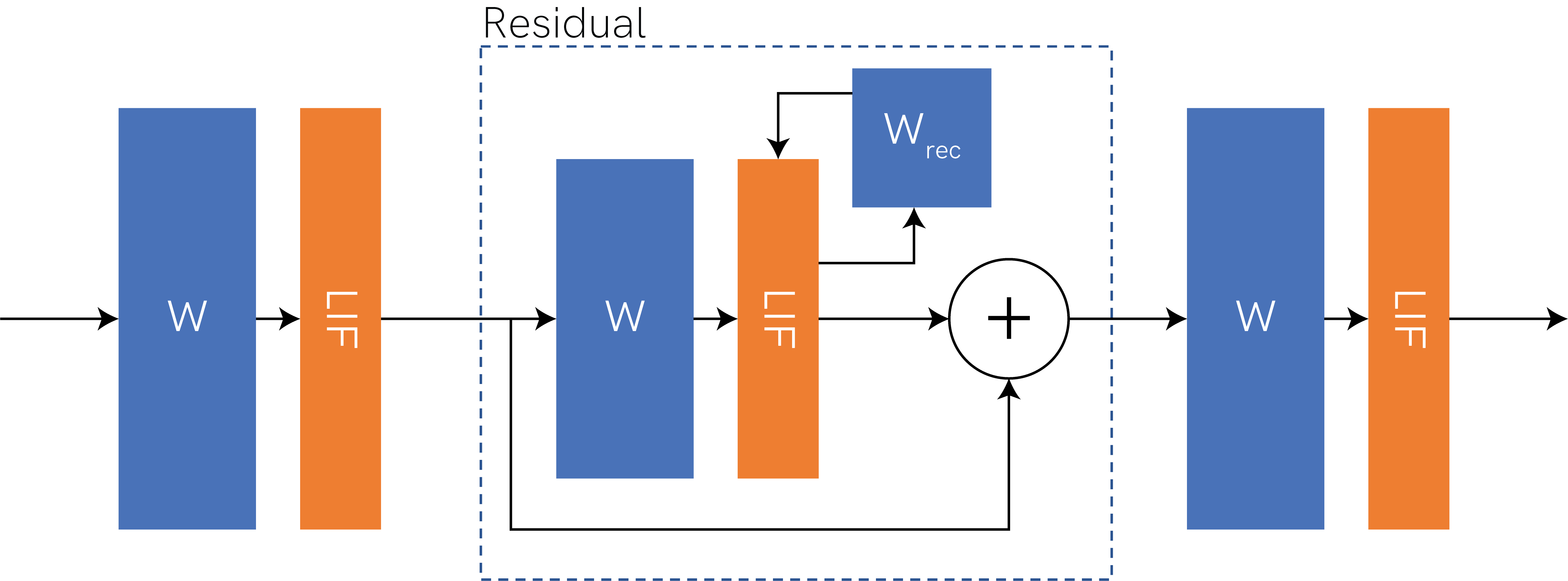
Step 1: Build a network in Rockpool

We will demonstrate with a straightforward network architecture, which shows off the support of Xylo. The network architecture is shown below. It consists of linear weights (“W”), spiking neuron layers (“LIF”), and a residual block containing a recurrent LIF layer (recurrent weights \(W_{rec}\)).

Image(filename='network-architecture.png')

# - Import the computational modules and combinators required for the networl
from rockpool.nn.modules import LIFTorch, LinearTorch
from rockpool.nn.combinators import Sequential, Residual

# - Define the size of the network layers
Nin = 2
Nhidden = 4
Nout = 2
dt = 1e-3

# - Define the network architecture using combinators and modules
net = Sequential(
    LinearTorch((Nin, Nhidden), has_bias = False),
    LIFTorch(Nhidden, dt = dt),

    Residual(
        LinearTorch((Nhidden, Nhidden), has_bias = False),
        LIFTorch(Nhidden, has_rec = True, threshold = 10., dt = dt),
    ),

    LinearTorch((Nhidden, Nout), has_bias = False),
    LIFTorch(Nout, dt = dt),
)
print(net)

TorchSequential  with shape (2, 2) {
    LinearTorch '0_LinearTorch' with shape (2, 4)
    LIFTorch '1_LIFTorch' with shape (4, 4)
    TorchResidual '2_TorchResidual' with shape (4, 4) {
        LinearTorch '0_LinearTorch' with shape (4, 4)
        LIFTorch '1_LIFTorch' with shape (4, 4)
    }
    LinearTorch '3_LinearTorch' with shape (4, 2)
    LIFTorch '4_LIFTorch' with shape (2, 2)
}

# - Scale down recurrent weights for stability
net[2][1].w_rec.data = net[2][1].w_rec / 10.

Step 2: Extract the computational graph for the network

To obtain a graph describing the entire network, which contains the computational flow of information through the network as well as all parameters, we simply use the as_graph() method.

For more information, see Computational graphs in Rockpool.

print(net.as_graph())

GraphHolder "TorchSequential__11277641184" with 2 input nodes -> 2 output nodes

Step 3: Map the network to a hardware specification

We now need to check that the network can be supported by the Xylo hardware, and assign hardware resources to the various aspects of the network architecture. For example, each neuron in the network must be assigned to a hardware neuron. Each non-input weight element in the network must be assigned to a global hidden weight matrix for Xylo. Output neurons in the final layer must be assigned to output channels.

The Xylo family includes sevral devices with differing HW blocks and support. These are supported by independent subpackages under rockpool.devices.xylo, and named after the chip ID in your HDK. Rockpool can detect this automatically for you, and import the correct package, by connecting to the HDK.

If you do not have a Xylo HDK, then you can use the rockpool.devices.xylo.syns61201 package supporting Xylo-Audio 2.

# - Import the Xylo HDK detection function
from rockpool.devices.xylo import find_xylo_hdks

# - Detect a connected HDK and import the required support package
connected_hdks, support_modules, chip_versions = find_xylo_hdks()

found_xylo = len(connected_hdks) > 0

if found_xylo:
    hdk = connected_hdks[0]
    x = support_modules[0]
else:
    assert False, 'This tutorial requires a connected Xylo HDK to run.'

The connected Xylo HDK contains a Xylo Audio v2 (SYNS61201). Importing `rockpool.devices.xylo.syns61201`

To convert the computational graph to a Xylo specfication, we use the mapper() function. In order to retain floating-point representations for parameters, we can specifiy weight_dtype = float. See the documentation for mapper() for further details.

# - Call the Xylo mapper on the extracted computational graph
spec = x.mapper(net.as_graph(), weight_dtype = 'float')

print(spec)

{
    'mapped_graph': GraphHolder "TorchSequential__11277641184" with 2 input nodes -> 2 output nodes,
    'weights_in': array([[-0.77903908,  1.18929613,  1.16114461,  0.22493351,  0.        ,
         0.        ,  0.        ,  0.        ],
       [ 1.32337248, -1.16171956, -1.33154929,  0.3293041 ,  0.        ,
         0.        ,  0.        ,  0.        ]]),
    'weights_out': array([[ 0.        ,  0.        ],
       [ 0.        ,  0.        ],
       [ 0.        ,  0.        ],
       [ 0.        ,  0.        ],
       [-0.84590757, -1.19352996],
       [-0.10860074,  0.6373018 ],
       [-0.16565597, -0.92963493],
       [-0.2262736 ,  0.42454898]]),
    'weights_rec': array([[ 0.        ,  0.        ,  0.        ,  0.        ,  0.10326695,
        -0.14892304,  1.01041162, -0.20021439],
       [ 0.        ,  0.        ,  0.        ,  0.        ,  0.03674126,
        -0.49414289, -0.6105172 ,  0.60044777],
       [ 0.        ,  0.        ,  0.        ,  0.        ,  0.34814227,
        -1.09550583,  0.31232011, -0.12054205],
       [ 0.        ,  0.        ,  0.        ,  0.        , -0.83039075,
         0.96797431, -0.54736292,  0.51089108],
       [ 0.        ,  0.        ,  0.        ,  0.        , -0.08836855,
         0.05024868,  0.09914371,  0.0179751 ],
       [ 0.        ,  0.        ,  0.        ,  0.        , -0.04342629,
         0.07340087,  0.05501813,  0.11716658],
       [ 0.        ,  0.        ,  0.        ,  0.        ,  0.0911395 ,
         0.1181069 ,  0.00574297,  0.06705973],
       [ 0.        ,  0.        ,  0.        ,  0.        , -0.03105988,
        -0.00630997,  0.07385659, -0.03389113]]),
    'dash_mem': array([4.32192802, 4.32192802, 4.32192802, 4.32192802, 4.32192802,
       4.32192802, 4.32192802, 4.32192802]),
    'dash_mem_out': array([4.32192802, 4.32192802]),
    'dash_syn': array([4.32192802, 4.32192802, 4.32192802, 4.32192802, 4.32192802,
       4.32192802, 4.32192802, 4.32192802]),
    'dash_syn_2': array([0., 0., 0., 0., 0., 0., 0., 0.]),
    'dash_syn_out': array([4.32192802, 4.32192802]),
    'threshold': array([ 1.,  1.,  1.,  1., 10., 10., 10., 10.]),
    'threshold_out': array([1., 1.]),
    'bias': array([0., 0., 0., 0., 0., 0., 0., 0.]),
    'bias_out': array([0., 0.]),
    'weight_shift_in': 0,
    'weight_shift_rec': 0,
    'weight_shift_out': 0,
    'aliases': [[4], [5], [6], [7], [], [], [], []],
    'dt': 0.001
}

Step 4: Quantize the specfication for the Xylo integer logic

Rockpool provides a number of functions for quantizing specifications for Xylo, in the package rockpool.transform.quantize_methods.

Here we will use global_quantize() to automatically find a good shared representation of the network parameters, that is compatible with the integer logic on Xylo.

from rockpool.transform import quantize_methods as q

# - Quantize the specification
spec.update(q.global_quantize(**spec))
print(spec)

{
    'mapped_graph': GraphHolder "TorchSequential__11277641184" with 2 input nodes -> 2 output nodes,
    'weights_in': array([[ -74,  113,  111,   21,    0,    0,    0,    0],
       [ 126, -111, -127,   31,    0,    0,    0,    0]]),
    'weights_out': array([[   0,    0],
       [   0,    0],
       [   0,    0],
       [   0,    0],
       [ -90, -127],
       [ -12,   68],
       [ -18,  -99],
       [ -24,   45]]),
    'weights_rec': array([[   0,    0,    0,    0,   10,  -14,   96,  -19],
       [   0,    0,    0,    0,    4,  -47,  -58,   57],
       [   0,    0,    0,    0,   33, -104,   30,  -11],
       [   0,    0,    0,    0,  -79,   92,  -52,   49],
       [   0,    0,    0,    0,   -8,    5,    9,    2],
       [   0,    0,    0,    0,   -4,    7,    5,   11],
       [   0,    0,    0,    0,    9,   11,    1,    6],
       [   0,    0,    0,    0,   -3,   -1,    7,   -3]]),
    'dash_mem': array([4, 4, 4, 4, 4, 4, 4, 4]),
    'dash_mem_out': array([4, 4]),
    'dash_syn': array([4, 4, 4, 4, 4, 4, 4, 4]),
    'dash_syn_2': array([0, 0, 0, 0, 0, 0, 0, 0]),
    'dash_syn_out': array([4, 4]),
    'threshold': array([ 95,  95,  95,  95, 954, 954, 954, 954]),
    'threshold_out': array([106, 106]),
    'bias': array([0, 0, 0, 0, 0, 0, 0, 0]),
    'bias_out': array([0, 0]),
    'weight_shift_in': 0,
    'weight_shift_rec': 0,
    'weight_shift_out': 0,
    'aliases': [[4], [5], [6], [7], [], [], [], []],
    'dt': 0.001
}

Step 5: Convert the specification to a hardware configuration

We now convert the network specification to a hardware configuration object for the Xylo HDK.

# - Use rockpool.devices.xylo.config_from_specification
config, is_valid, msg = x.config_from_specification(**spec)
if not is_valid:
    print(msg)

Step 6: Deploy the configuration to the Xylo HDK

# - Use rockpool.devices.xylo.XyloSamna to deploy to the HDK
if found_xylo:
    modSamna = x.XyloSamna(hdk, config, dt = dt)
    print(modSamna)

XyloSamna  with shape (2, 8, 2)

Step 7: Evolve the network on the Xylo HDK

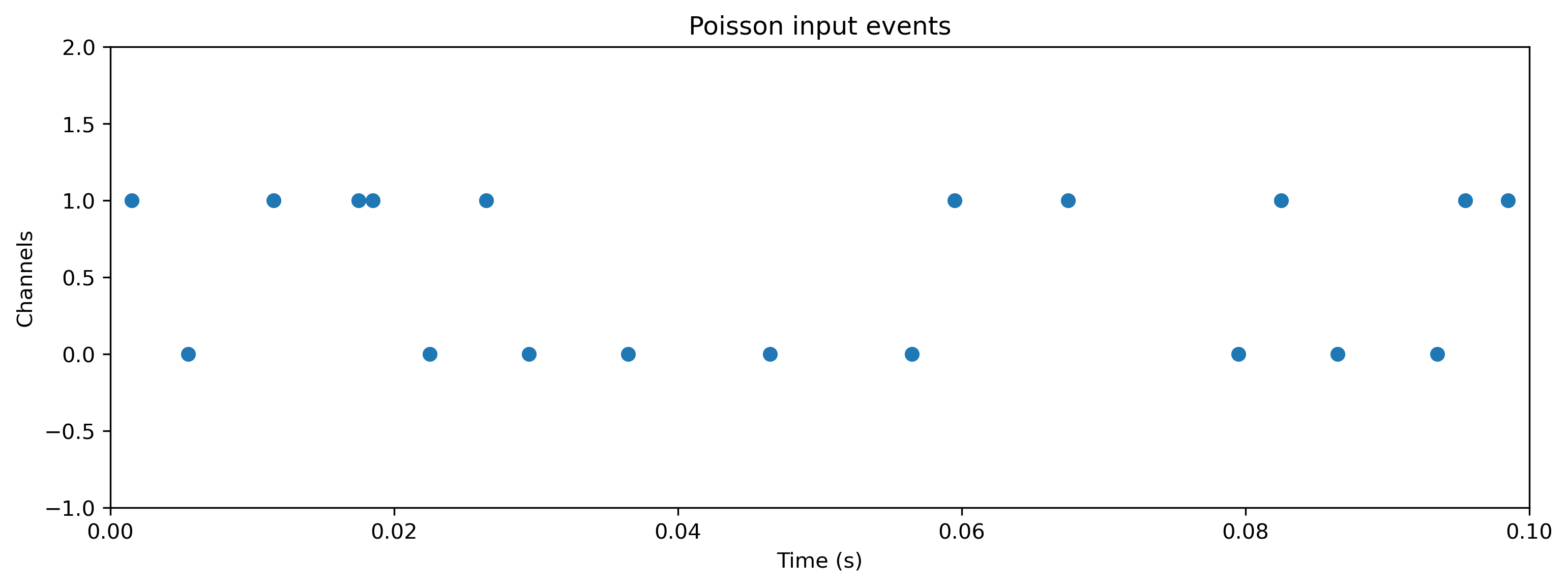
Now we will generate a random Poisson input, and evolve the network on the Xylo HDK using this input. Using Rockpool we can record all internal states on the Xylo HDK during evolution. Note that recording internal state slows evolution below real-time.

# - Generate some Poisson input
T = 100
f = 0.1
input_spikes = np.random.rand(T, Nin) < f
TSEvent.from_raster(input_spikes, dt, name = 'Poisson input events').plot();

# - Evolve the network on the Xylo HDK
if found_xylo:
    out, _, r_d = modSamna(input_spikes, record = True)

    # - Show the internal state variables recorded
    print(r_d.keys())

dict_keys(['Vmem', 'Isyn', 'Isyn2', 'Spikes', 'Vmem_out', 'Isyn_out', 'times'])

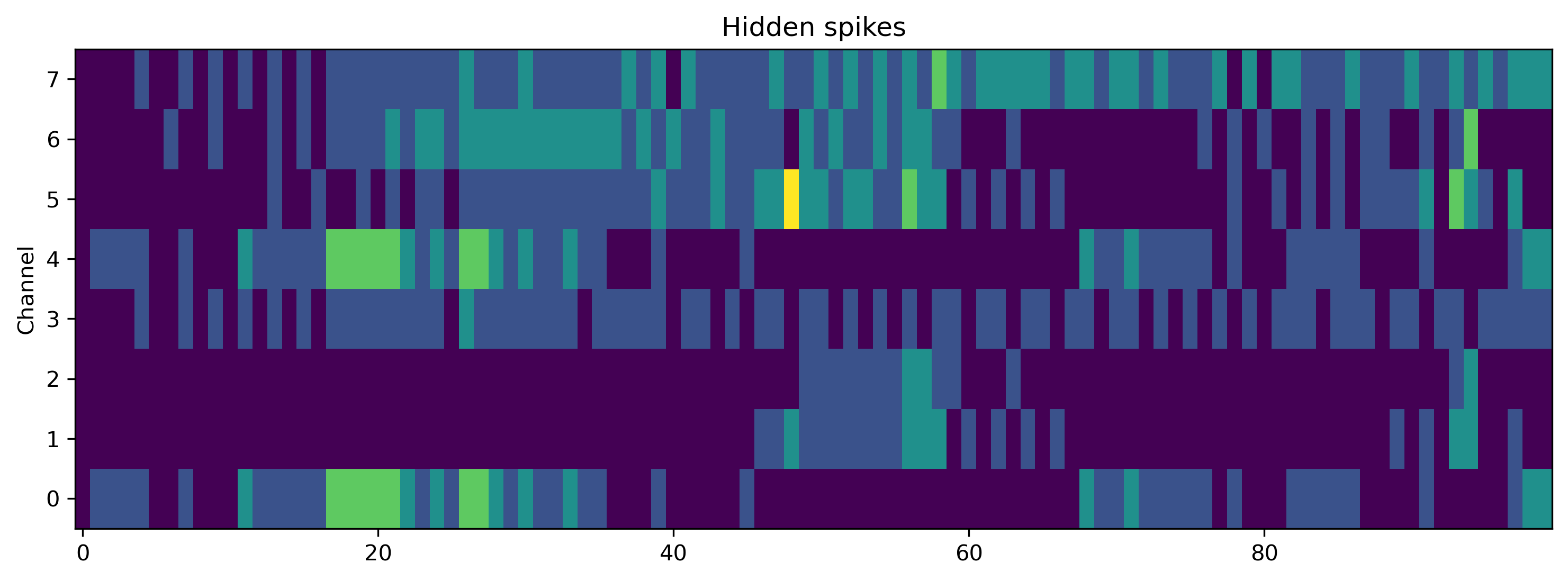
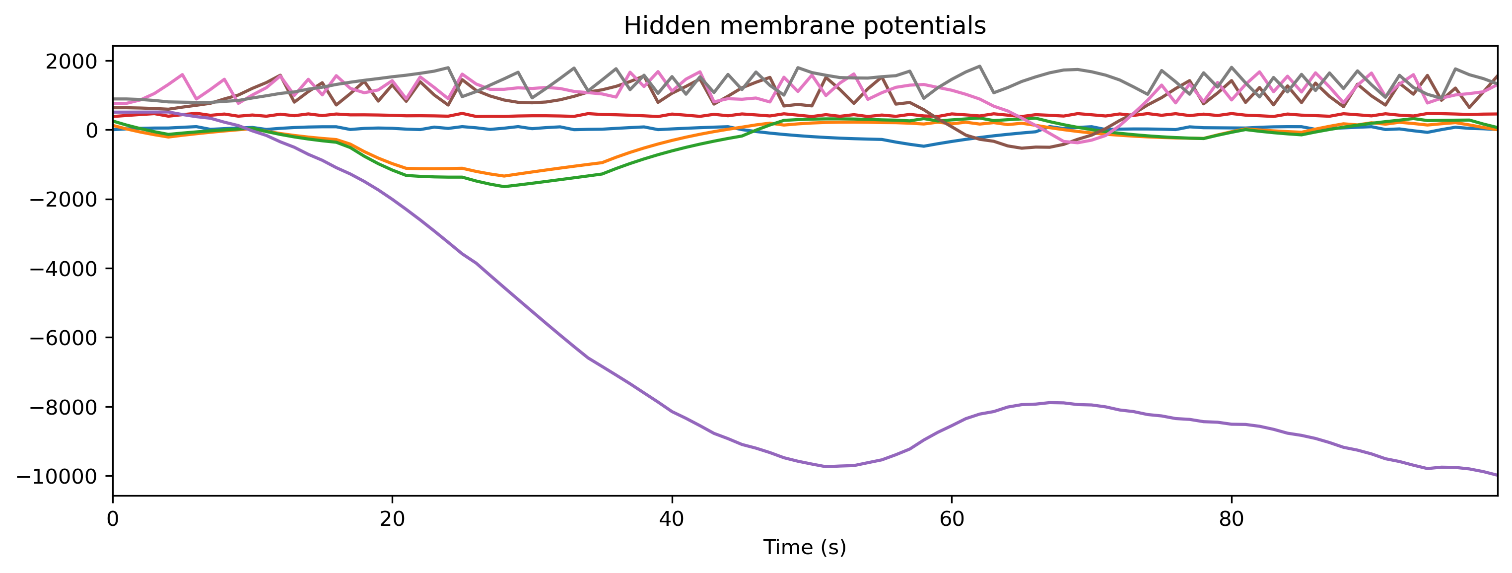
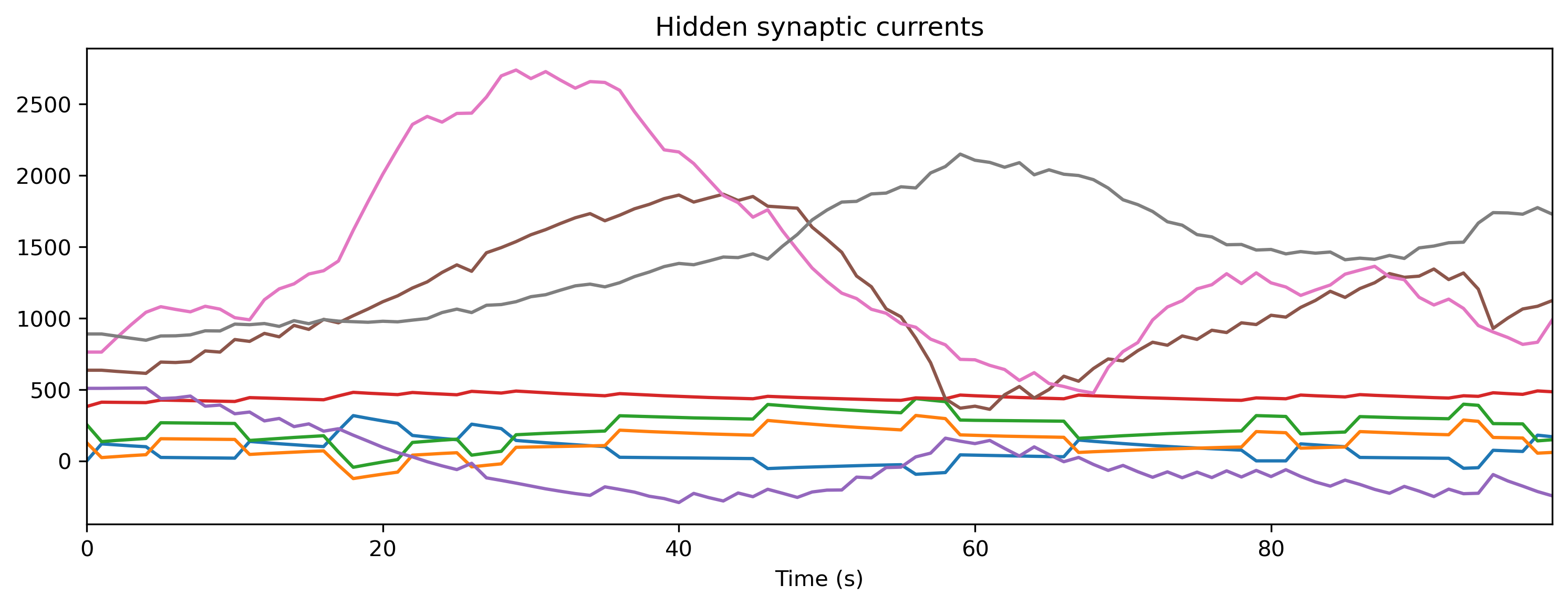
# - Plot some internal state variables
if found_xylo:
    plt.figure()
    plt.imshow(r_d['Spikes'].T, aspect = 'auto', origin = 'lower')
    plt.title('Hidden spikes')
    plt.ylabel('Channel')

    plt.figure()
    TSContinuous(r_d['times'], r_d['Vmem'], name = 'Hidden membrane potentials').plot(stagger = 127)

    plt.figure()
    TSContinuous(r_d['times'], r_d['Isyn'], name = 'Hidden synaptic currents').plot(stagger = 127)

Step 8: Simulate the HDK using a bit-precise simulator

Rockpool comes bundled with XyloSim, a bit-precise simulator of the Xylo SNN core. The interface to evolve and record from a XyloSim object is identical to other Rockpool modules.

We create a XyloSim object using the same hardware configuration that we used to deploy the network to the Xylo HDK.

modSim = x.XyloSim.from_config(config)
print(modSim)

XyloSim  with shape (16, 1000, 8)

# - Evolve the input over the network, in simulation
out, _, r_d = modSim(input_spikes, record = True)

# - Show the internal state variables recorded
print(r_d.keys())

dict_keys(['Vmem', 'Isyn', 'Isyn2', 'Spikes', 'Vmem_out', 'Isyn_out'])

# - Plot some internal state variables
plt.figure()
plt.imshow(r_d['Spikes'].T, aspect = 'auto', origin = 'lower')
plt.title('Hidden spikes')
plt.ylabel('Channel')

plt.figure()
TSContinuous.from_clocked(r_d['Vmem'], dt, name = 'Hidden membrane potentials').plot(stagger = 127)

plt.figure()
TSContinuous.from_clocked(r_d['Isyn'], dt, name = 'Hidden synaptic currents').plot(stagger = 127);

If you compare the traces here with those recorded from the Xylo HDK above, you will see they are identical. XyloSim provides a way to quickly verify a network configuration without requiring the Xylo HDK hardware.

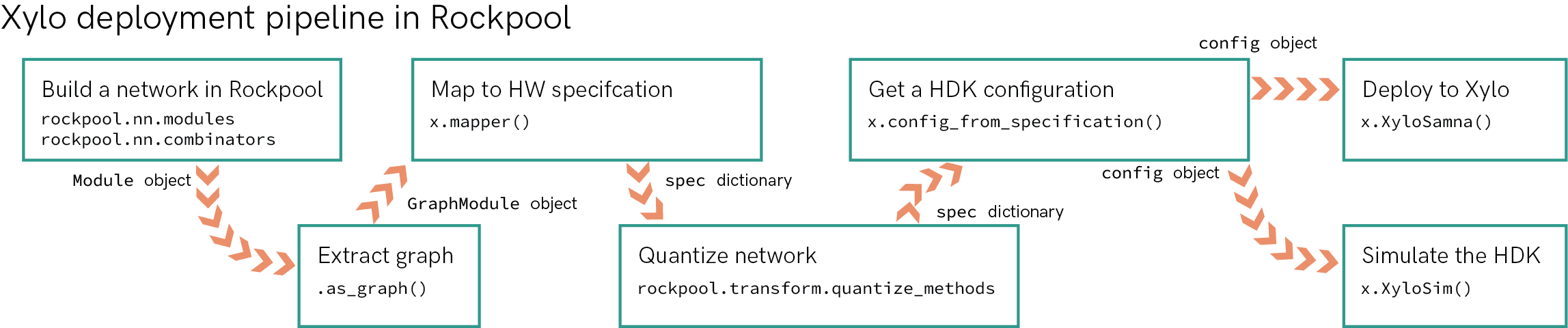
Summary

The flow-chart below summarises the steps in taking a Rockpool network from a high-level definition to deployment on the Xylo HDK.

Image(filename='xylo-pipeline.png')