This page was generated from docs/devices/xylo-a3/Using_XyloSamna_and_XyloMonitor.ipynb. Interactive online version:

Using XyloSamna and XyloMonitor to deploy a model on XyloAudio 3 HDK

In this tutorial, we go through an example of deploying an audio classification model (trained in Rockpool) into XyloAudio 3 SNN core in two modes:

• Accelerated time mode using XyloSamna

• Real-time mode using XyloMonitor

Accelerated time mode is recommended to check the trained model’s validity quickly. Before running the pipeline in real-time, the user can test the model by bypassing the microphone in Accelerated time mode and feeding pre-recorded spike trains.

In Real-time mode, the model will be mapped to the Xylo SNN core and run in real time, with live microphone input. This mimics the deployment of an application in a real system.

The steps for deploying a model are as follows:

1. Load, map, and quantize the trained checkpoint with tools and transforms from Rockpool

2. Build the configuration object for the SNN core

For Accelerated time mode:

3. Instantiate a XyloSamna by passing the configuration object and the connected Xylo HDK device

4. Feed the input (pre-generated spike train)

5. Analyze the output of the SNN core

For Real-time mode:

3. Instantiate a XyloMonitor by passing the configuration object and the connected Xylo HDK device

4. Play the audio files and record the output of SNN Core

Common steps for both Accelerated and Real-time mode

Loading the trained model

In this example, we use a trained model for a multiclass classification task: detecting rare sounds like glass-break, gun-shot, scream, and background noise. The model was trained using the Mivia Audio Events Dataset: https://mivia.unisa.it/datasets/audio-analysis/mivia-audio-events/. The model is composed of 16 input channels, three layers of Leaky Integrate-and-Fire (LIF) neurons, and four output neurons, one for each class.

from rockpool.nn.networks import SynNet
from rockpool.nn.modules import LIFTorch
import warnings
warnings.filterwarnings("ignore")

ckpt = 'model_sample/to_deploy_inXylo.json'

#  trained model architecture parameters
arch_params = {'n_classes': 4,
'n_channels': 16,
'size_hidden_layers':[63, 63, 63],
'time_constants_per_layer':[3,7,7],
'tau_syn_base': 0.02,
'tau_mem': 0.02,
'tau_syn_out': 0.02,
'neuron_model': LIFTorch,
'dt': 0.00994,
'output': 'vmem'}

# Number of input channels
Nin = 16
model_dt = 0.009994

# instantiating the model backbone and loading trained checkpoint
model = SynNet(** arch_params)
model.load(ckpt)

WARNING    /home/karlaburelo/Tools/rockpool/rockpool/nn/networks/__init__.py:15: UserWarning: This module needs to be ported to the v2 API.
  warnings.warn(f"{err}")
 [py.warnings]
WARNING    /home/karlaburelo/Tools/rockpool/rockpool/nn/networks/__init__.py:20: UserWarning: This module needs to be ported to the v2 API.
  warnings.warn(f"{err}")
 [py.warnings]

Mapping, quantizing and building the configuration object for XyloAudio 3 HDK

from rockpool.devices.xylo.syns65302 import config_from_specification, mapper
import rockpool.transform.quantize_methods as q

# getting the model specifications using the mapper function
spec = mapper(model.as_graph(), weight_dtype='float', threshold_dtype='float', dash_dtype='float')
# quantizing the model
spec.update(q.channel_quantize(**spec))

xylo_conf, is_valid, msg = config_from_specification(**spec)

Using XyloSamna in Accelerated time mode

In Accelerated time mode we can give a specific input to XyloAudio that will be processed as quickly as possible, while allowing the monitoring of the internal network state. This mode is ideal for benchmarking and validating models.

In Accelerated time, the input has to be a list of spike events ordered by timestep.

Creating XyloSamna: API to interact with HDK in Accelerated time mode

Note: We need an AudioXylo 3 connected to run this step

from rockpool.devices.xylo.syns65302 import xa3_devkit_utils as hdu
from rockpool.devices.xylo.syns65302 import XyloSamna
import samna

# Getting the connected devices and choosing XyloAudio 3 board
xylo_nodes = hdu.find_xylo_a3_boards()

if len(xylo_nodes) == 0:
    raise ValueError('A connected XyloAudio 3 development board is required for this tutorial.')

xa3 = xylo_nodes[0]

# Instantiating XyloSamna and deploying to the dev kit; make sure your dt corresponds to the dt of your input data
Xmod = XyloSamna(device=xa3, config=xylo_conf, dt = model_dt)

Feeding test samples of rare-sounds to XyloSamna and analyzing recorded states

• Please see this tutorial as an example on how to convert audio signals into spike trains.

import numpy as np
import matplotlib.pyplot as plt

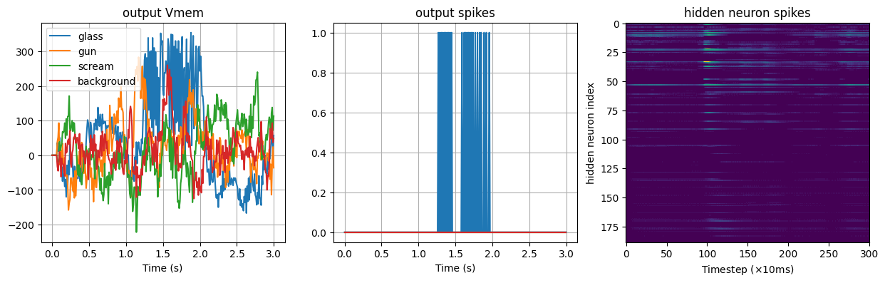
rare_sounds = ['glass', 'gun', 'scream', 'background']

for sound in rare_sounds:
    print(f'Testing {sound} sound')
    test_sample = np.load(f'afesim_sample/AFESimExternalSample_{sound}.npy', allow_pickle=True)
    # with XyloSamna we can record the internal state of the network
    out, _, rec = Xmod(test_sample, record=True)
    prediction = rare_sounds[np.argmax(np.sum(out, axis = 0))]
    print(f'Detected sound: {prediction} \n')

    # Show internal states
    plt.figure(figsize=(15,4))
    plt.subplot(131); plt.plot(rec['times'], rec['Vmem_out'], label = rare_sounds);plt.legend(), plt.grid(True); plt.xlabel('Time (s)'); plt.title('output Vmem');
    plt.subplot(132); plt.plot(rec['times'], out);plt.grid(True); plt.xlabel('Time (s)'); plt.title('output spikes');
    plt.subplot(133); plt.imshow(rec['Spikes'].T, aspect='auto', interpolation='none'); plt.xlabel('Timestep ($\\times$10ms)'); plt.ylabel('hidden neuron index'); plt.title('hidden neuron spikes');
    plt.show()

del Xmod

Testing glass sound
Detected sound: glass

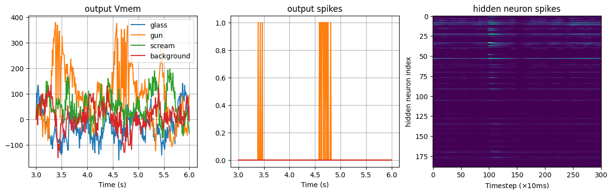
Testing gun sound
Detected sound: gun

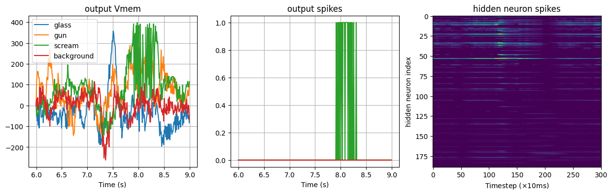
Testing scream sound
Detected sound: scream

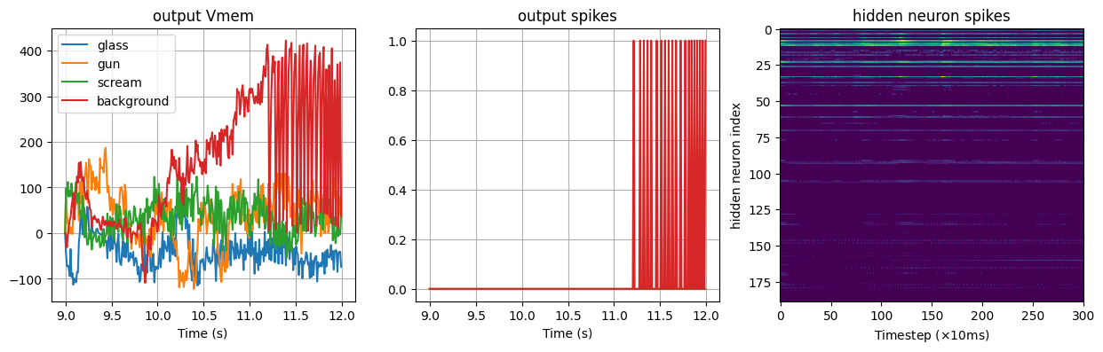
Testing background sound
Detected sound: background

Using XyloMonitor in Real Time mode

In Real-time mode, XyloAudio 3 continuously processes events as they are received. Events are received directly from one of the onboard microphones instead of event-based input.

In this mode, the chip operates autonomously, collecting inputs and processing them. Once the processing is done, XyloAudio 3 outputs all generated spike events. It is not possible to interact with the chip during this period. Thus, the collection of internal neuron states is not permitted.

Creating XyloMonitor: API to interact with HDK in Real-time mode

XyloMonitor uses the XyloAudio 3 embedded microphone to feed input to the SNN Core. We will use the previously created configuration object to instantiate XyloMonitor and test it by playing an audio file.

Note: We need an AudioXylo 3 connected to run this step

import samna
from rockpool.devices.xylo.syns65302 import xa3_devkit_utils as hdu
from rockpool.devices.xylo.syns65302 import XyloMonitor

from scipy.io import wavfile
!pip install simpleaudio
import simpleaudio as sa
import numpy as np

def get_wave_object(test_file):
    sample_rate, data = wavfile.read(test_file)

    duration = int(len(data)/sample_rate) # in seconds
    n = data.ndim

    if data.dtype == np.int8:
        bytes_per_sample = 1
    elif data.dtype == np.int16:
        bytes_per_sample = 2
    elif data.dtype == np.float32:
        bytes_per_sample = 4
    else:
        raise ValueError("recorded audio should have 1 or 2 bytes per sample!")

    wave_obj = sa.WaveObject(
        audio_data= data,
        num_channels=data.ndim,
        bytes_per_sample=bytes_per_sample,
        sample_rate=sample_rate
    )

    return duration,wave_obj

Warning: The next cell will play an audio sample for each class (glass-break, gun-shot, scream, background). If you would like to test the detection using the XYloAudio development board, make sure the microphone on the board is close to your PC speaker, at a reasonable volume.

for sound in rare_sounds:
    print(f'Testing {sound} sound')
    # Load audio sample
    test_audio = f'audio_sample/{sound}_sample.wav'
    duration, wave_obj = get_wave_object(test_audio)
    T = int(duration/model_dt) # timesteps

    # Instantiate XyloMonitor, deploy network to device
    xylo_monitor  = XyloMonitor(device=xa3, config=xylo_conf, dt = model_dt, output_mode='Spike', dn_active = True, main_clk_rate=12.5)

    # Evolve XyloMonitor object
    play_obj = wave_obj.play()
    out, state, rec = xylo_monitor.evolve(input_data=np.zeros([T, Nin]), record_power=True)
    play_obj.wait_done()

    # Prediction
    prediction = rare_sounds[np.argmax(np.sum(out, axis = 0))]
    print(f'Detected sound: {prediction} \n')
    del xylo_monitor

Testing glass sound
Detected sound: glass

Testing gun sound
Detected sound: gun

Testing scream sound
Detected sound: scream

Testing background sound
Detected sound: background

Power consumption

We can record the power consumption by setting ``record_power = True`` while evolving with :py:class:`~.syns65302.XyloMonitor`. This will record the power in the three channels: ``io``, ``analog`` and ``digital``. Note: we can configure the chip to run with a slower clock to save energy. Note, however, that we need to use a clock speed that is fast enough to finish the data processing in one step.

io_power = np.mean(rec['io_power'])
analog = np.mean(rec['analog_power'])
digital = np.mean(rec['digital_power'])

print(f'XyloAudio 3\nio:\t{np.ceil(io_power * 1e6):.0f} µW\tAFE core:\t{np.ceil(analog * 1e6):.0f} µW\tDFE+SNN core:\t{np.ceil(digital * 1e6):.0f} µW\n')

XyloAudio 3
io:     456 µW  AFE core:       13 µW   DFE+SNN core:   612 µW