This page was generated from docs/devices/xylo-overview.ipynb. Interactive online version:

🐝 Overview of the Xylo™ family

Xylo™ is a family of ultra-low-power (sub-mW) sensory processing and classification devices, relying on efficient spiking neural networks for inference. The Xylo SNN core is an efficient digital simulator of spiking leaky integrate-and-fire neurons with exponential input synapses. Xylo is highly configurable, and supports individual synaptic and membrane time-constants, thresholds and biases for each neuron. Xylo supports arbitrary network architectures, including recurrent networks, residual spiking networks, and more.

Xylo is currently available in several versions with varying HW support and front-ends.

Family design

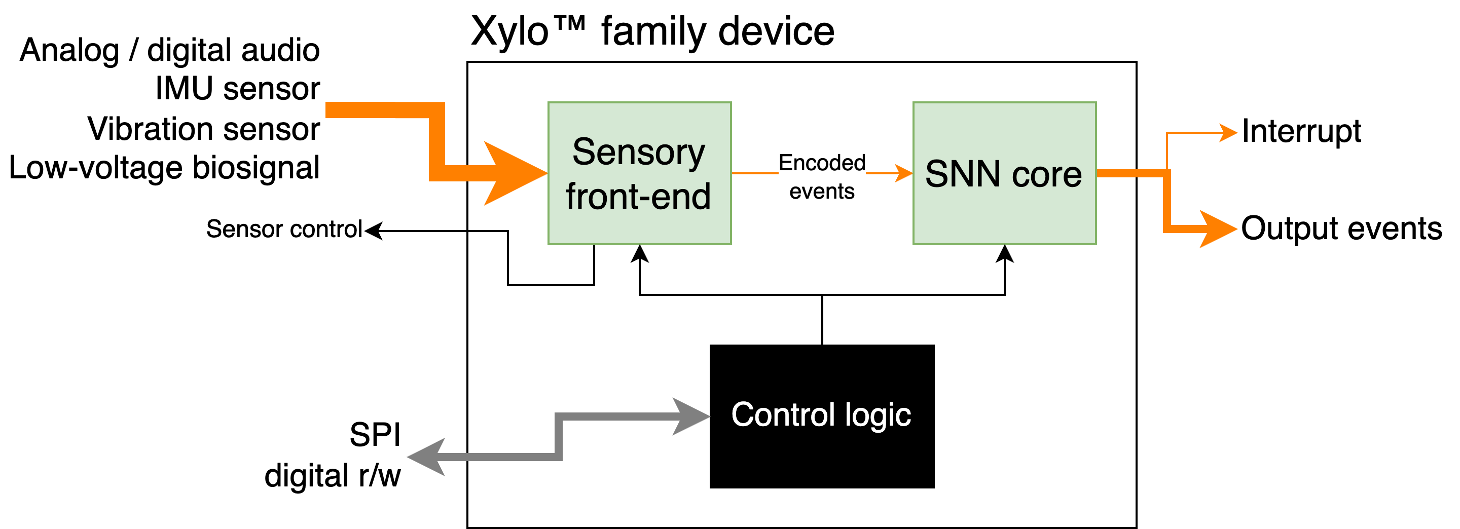
Xylo™ devices comprise an efficient sensory encoding front-end, a Xylo SNN inference core with on-board memory, and control logic. The various devices in the family interface directly with analog and digital audio sensors (Xylo™Audio); IMU motion devices (Xylo™IMU); and other sensory input modalities.

from IPython.display import Image
Image("images/xylo_family-overview.png")

Xylo family members

Device name	XyloAudio 2	XyloAudio 3	XyloIMU
Quick-start docs	🐝🎵 Introduction to Xylo™Audio	🐝⚡️ Quick start with Xylo™Audio 3	🐝💨 Introduction to Xylo™IMU
Input sensor	Analog microphone	Digital microphone	MEMS 3-channel IMU
Num. sensor channels	1	1	3 (x, y, z)
Num. SNN input channels	16	16	16
Num. hidden neurons	1000	992	496
Num. Syn. states	2	2	1
Num. output neurons	8	32	16
Max. fanout	64	1024	512
Avg. fanout	32+32 (Syn1 and Syn2)	32+32 (Syn1 and Syn2)	64
Max. input projection	to 1000 hidden neurons	to 128 hidden neurons	to 128 hidden neurons
Max. output projection	from 1000 hidden neurons	from 128 hidden neurons	from 128 hidden neurons

SNN core logical architecture

The figure below shows the overall logical architecture of Xylo. It is designed to support deployment of arbitrary SNN architectures, including recurrent, block-recurrent spiking residual and other compex network architectures.

Image("images/xylo_network-architecture.png")

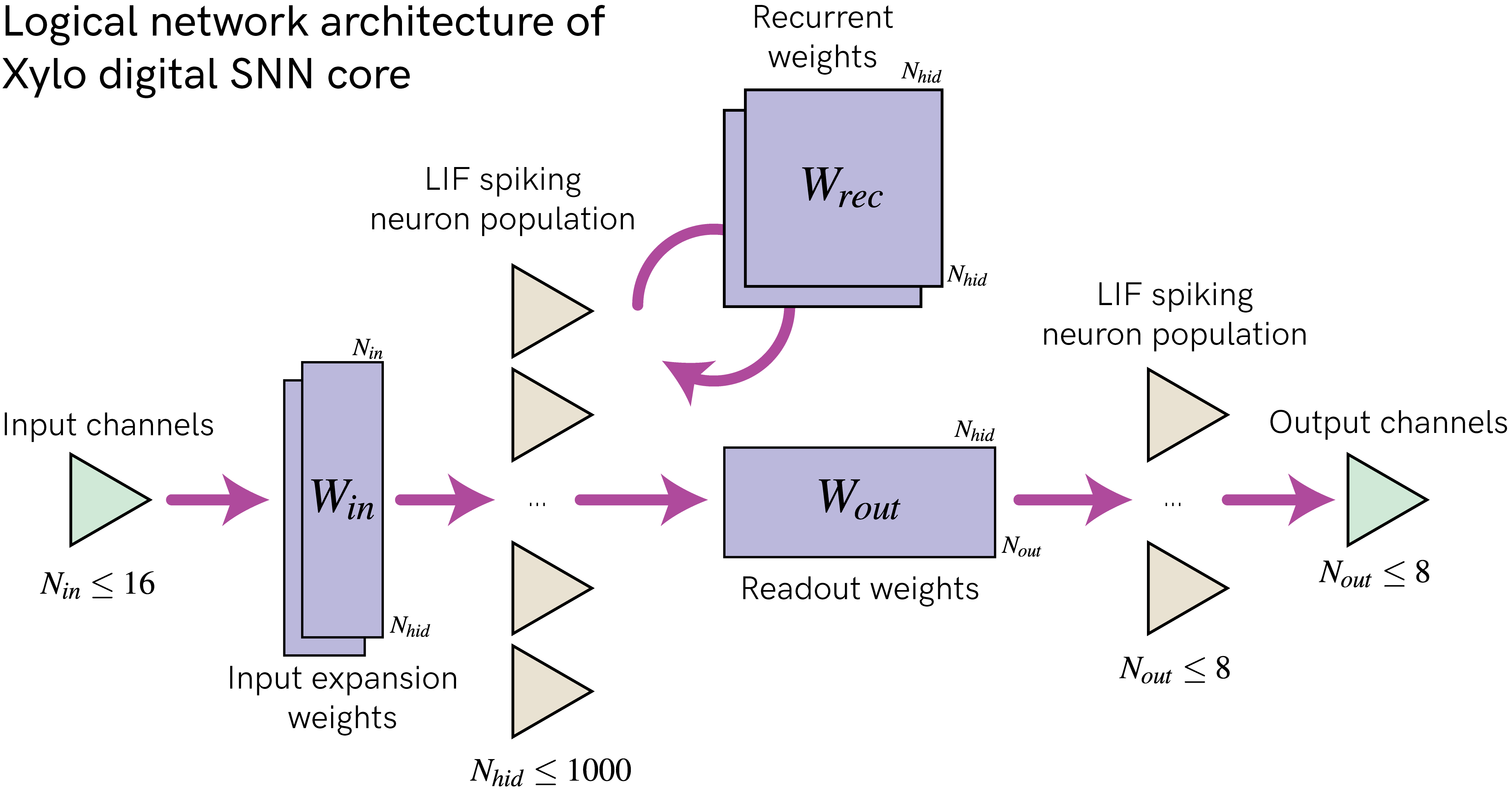
• Synchronous time-stepped architecture with a global time-step dt

• Up to 16 event-based input channels, supoorting up to 15 input events per time-step per channel

• 8-bit input expansion weights \(W_{in}\)

• Up to \(N_{hid} = 1000\) digital LIF hidden neurons, depending on device (see below for neuron model)

  • one or two available input synapses, depending on device

  • bit-shift decay on synaptic and membrane potentials

  • Independently chosen time constants and thresholds per neuron

  • Subtractive reset, with up to 31 events generated per time-step per neuron

• 8-bit recurrent weights \(W_{rec}\) for connecting the hidden population

• 1 output alias supported for each hidden neuron -> copies the output events to another neuron

• 8-bit readout weights \(W_{out}\)

• Up to \(N_{out} = 32\) digital LIF readout neurons, depending on device

  • same neuron model as hidden neurons

  • only one available input synapse

  • only one event generated per time-step per neuron

Image("images/xylo_neuron-model.png")

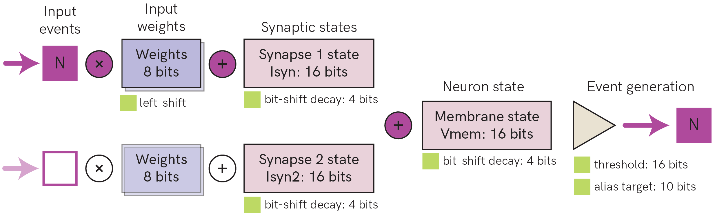
The figure above shows the digital neuron model and parameters supported on Xylo Audio 2 and 3. Other devices in the Xylo family support only one synaptic state per neuron. See the detailed documentation for each device for further information.

• Up to 15 input spikes are supported per time step for each input channel

• Each hidden layer neuron supports up to two synaptic input states. Output layer neurons support only one synaptic input state

• Synaptic and neuron states undergo bit-shift decay as an approximation to exponential decay. Time constants of decay are individually configurable per synapse and per neuron.

• Multiple events can be generated on each time-step, if the threshold is exceeded multiple times. Up to 31 spikes can be generated on each time-step.

• Output neurons can only generate one event per time-step

• Reset during event generation is performed by subtraction

• Hidden neurons have a limited average fan-out, depending on the weight resources available on the Xylo device

# - Switch off warnings
import warnings

warnings.filterwarnings("ignore")

# - Useful imports
import sys
!{sys.executable} -m pip install --quiet matplotlib
import matplotlib.pyplot as plt

%matplotlib inline
plt.rcParams["figure.figsize"] = [12, 4]
plt.rcParams["figure.dpi"] = 300

try:
    from rich import print
except:
    pass

import numpy as np

Bit-shift decay

Xylo devices simulate exponential decay using an efficient bit-shift-subtraction technique. Consequently, time constants are expressed as “bit-shift decay” parameters (“dash” parameters) which are a function of the fixed simulation time-step. The equation for that conversion is:

\(dash = [\log_2(\tau / dt)]\)

Hence, the dash parameter for a synapse with a 2 ms time constant, with a simulation resolution of 1 ms, is 1.

But what is done with this bitshift of 1? Let’s compare exponential decay with bitshift decay. The bit-shifting decay method is illustrated by the function bitshift() below.

def bitshift(value: int, dash: int) -> int:
    # - Bit-shift decay
    new_value = value - (value >> dash)

    # - Linear decay below dash-driven change
    if new_value == value:
        new_value -= 1

    return new_value

As you can see, the bit-shifting decay is accomplished by the line

\(v' = v - (v >> dash)\)

where \(>>\) is the right-bit-shift operator; \(v\) is the current value and \(v'\) is the new value after the bit-shifting step. Since \(v\) is an integer, for low values of \(v\), \(v >> dash = 0\). We therefore perform a linear decay for low values of \(v\).

def plot_tau_dash(tau: float, dt_: float = 1e-3, simtime: float = None):
    if simtime is None:
        simtime = tau * 10.0

    # - Compute dash, and the exponential propagator per time-step
    dash = np.round(np.log2(tau / dt_)).astype(int)
    exp_propagator = np.exp(-dt_ / tau)

    # - Compute exponential and dash decay curves over time
    t_ = 0
    v_tau = [1000]
    v_dash = [1000]
    while t_ < simtime:
        v_tau.append(v_tau[-1] * exp_propagator)
        v_dash.append(bitshift(v_dash[-1], dash))
        t_ += dt_

    # - Plot the two curves for comparison
    plt.plot(
        np.arange(0, len(v_tau)) * dt_ * 1e3,
        v_tau,
        label=f"exponential decay, $\\tau$={int(tau * 1e3)}ms",
    )
    plt.plot(
        np.arange(0, len(v_dash)) * dt_ * 1e3,
        v_dash,
        "--",
        label=f"bitshift decay, dash={dash}",
    )
    plt.legend()
    plt.xlabel("Time (ms)")


# - Plot examples for tau = 16ms and tau = 25 ms
plt.figure()
plt.subplot(1, 2, 1)
plot_tau_dash(16e-3)

plt.subplot(1, 2, 2)
plot_tau_dash(25e-3)

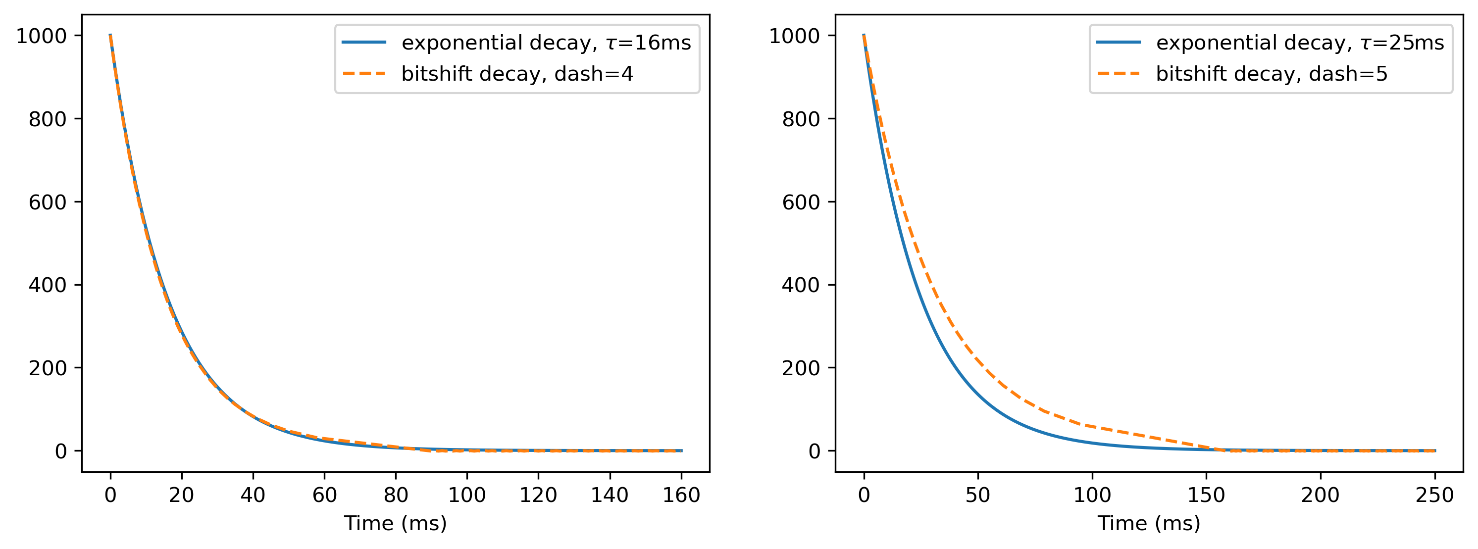
For powers of two, the approximation is very close. But since this is integer arithmetic, the approximation will not always be perfect. We can see this with the example of \(\tau = 25\)ms.

Next steps

For information about setting up a Xylo simulation and deploying to a Xylo HDK, see 🐝⚡️ Quick-start with Xylo SNN core

For an introduction to audio processing with Xylo Audio 2, see 🐝🎵 Introduction to Xylo™Audio

For an introduction to audio processing with Xylo Audio 3, see 🐝⚡️ Quick start with Xylo™Audio 3

For an overview of Xylo IMU, see 🐝💨 Introduction to Xylo™IMU