This page was generated from docs/in-depth/jax-training.ipynb. Interactive online version:

🏃🏽‍♀️ Training a Rockpool network with Jax

Jax is a Python package for differentiable programming. With a convenient numpy-like interface, Jax will automagically compute the gradients of your code. This is a huge boon for optimisation, especially for neural networks.

In this overview we show how to build and optimise a simple Jax-based network in Rockpool. We show how to write a task Dataset, how to write a loss function, and how to write a training loop to perform the optimisation.

We also illustrate some advanced topics, such as providing parameter bounds during optimisation.

# -- Some useful imports

# - Switch off warnings
import warnings

warnings.filterwarnings("ignore")

# - Rich printing
try:
    from rich import print
except:
    pass

# - Numpy
import numpy as np

# - Import and configure matplotlib for plotting
import sys
!{sys.executable} -m pip install --quiet matplotlib
import matplotlib.pyplot as plt

%matplotlib inline
plt.rcParams["figure.figsize"] = [12, 4]
plt.rcParams["figure.dpi"] = 300

Jax considerations

Jax is a functional programming library — ideally everything should be written as side-effect-free functions. For this purpose, Rockpool provides the functional API (see [𝝺] Low-level functional API). Rockpool tries to make using Jax-backed modules as straightforward as possible, via the JaxModule base class.

Jax provides a very convenient numpy-compatible interface, via the jax.numpy package. If you need to do any numeric computation interfaced with Rockpool/Jax, then you must use jax.numpy. You’ll receive an error if you don’t.

Loss functions

Loss function components provided by Rockpool

Rockpool provides some useful training utilities under training. training.jax_loss includes several components for building your own loss (or cost) functions.

Function	Use
mse()	Mean-squared error (basic loss). Ensures that two signals become more similar (e.g. target signal and network output).
l2sqr_norm()	L2-squared norm, for parameter regularisation. Keeps parameter values closer to zero.
l0_norm_approx()	Smooth and differentiable L0 norm approximation. Encourages parameter sparsity (i.e. many zero entries in a parameter vector).
bounds_cost()	Provide a cost function component that enforces minimum and/or maximum parameter bounds.
make_bounds()	Convenience function to construct a template set of bounds for use in an optimisation problem.
softmax()	Compute the softmax function. Useful for incorporation in the readout layers of deep networks, during training.
logsoftmax()	Compute the log softmax function. Used in readouts when training with cross-entopy loss functions.

You can use these components by importing rockpool.training.jax_loss:

# - Import the loss components for use
from rockpool.training import jax_loss as l

Writing your own loss function

For later use in optimising a network, a loss function must be differentiable with respect to the network parameters. A convenient way to achieve this is illutrated here, where we define a loss function that accepts the parameters, the network object, the inputs for this batch, and the corresponding target signals.

The loss function is then responsible for initialising the network — remember Rockpool networks usually have state, and this needs to be taken into account during training – setting the network parameters, evolving the network and computing the loss for this batch.

This form is convenient since you can compute gradients over the entire function. By default, jax computes gradients over the first argument to a function — in this case, the set of network parameters.

Remember, if you want to do any other arbitrary calculations, you must use jax.numpy instead of numpy.

def loss_mse(parameters, net, inputs, target):
    # - Handle the network state — randomise or reset
    net = net.reset_state()

    # - Assign the provided parameters to the network
    net = net.set_attributes(parameters)

    # - Evolve the network to get the ouput
    output, _, _ = net(inputs)

    # - Compute a loss value w.r.t. the target output
    return l.mse(output, target)

Defining a task dataset

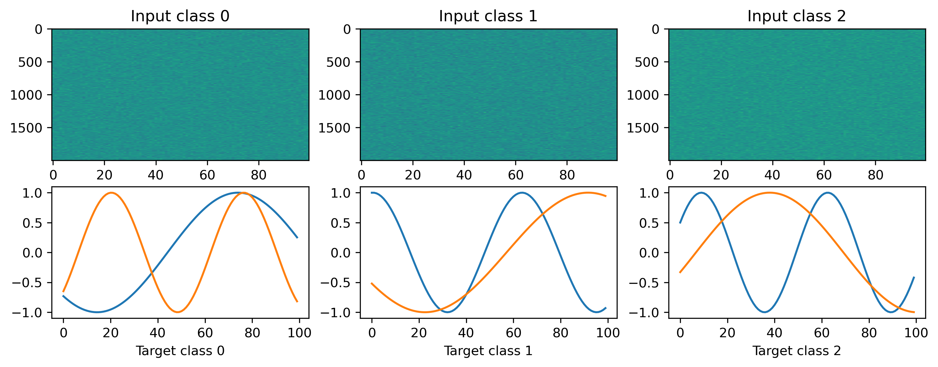
We will define a simple random regression task, where random frozen input noise is mapped to randomly chosen smooth output signals. We implement this using a Dataset-compatible class, implementing the __len__() and __getitem__() methods.

# - Define a dataset class implementing the indexing interface
class MultiClassRandomSinMapping:
    def __init__(
        self,
        num_classes: int = 2,
        sample_length: int = 100,
        input_channels: int = 50,
        target_channels: int = 2,
    ):
        # - Record task parameters
        self._num_classes = num_classes
        self._sample_length = sample_length

        # - Draw random input signals
        self._inputs = np.random.randn(num_classes, sample_length, input_channels) + 1.0

        # - Draw random sinusoidal target parameters
        self._target_phase = np.random.rand(num_classes, 1, target_channels) * 2 * np.pi
        self._target_omega = (
            np.random.rand(num_classes, 1, target_channels) * sample_length / 50
        )

        # - Generate target output signals
        time_base = np.atleast_2d(np.arange(sample_length) / sample_length).T
        self._targets = np.sin(
            2 * np.pi * self._target_omega * time_base + self._target_phase
        )

    def __len__(self):
        # - Return the total size of this dataset
        return self._num_classes

    def __getitem__(self, i):
        # - Return the indexed dataset sample
        return self._inputs[i], self._targets[i]

# - Instantiate a dataset
Nin = 2000
Nout = 2
num_classes = 3
T = 100
ds = MultiClassRandomSinMapping(
    num_classes=num_classes,
    input_channels=Nin,
    target_channels=Nout,
    sample_length=T,
)

# Display the dataset classes
plt.figure()
for i, sample in enumerate(ds):
    plt.subplot(2, len(ds), i + 1)
    plt.imshow(sample[0].T, aspect="auto")
    plt.title(f"Input class {i}")

    plt.subplot(2, len(ds), i + len(ds) + 1)
    plt.plot(sample[1])
    plt.xlabel(f"Target class {i}")

Building a Jax network

We’ll define a very simple network to solve the regression task, which will in fact not be stateful — we’ll use LinearJax modules to wrap weight matrices, and the InstantJax module to add a non-linearity.

We’ll build an MLP-like network with one hidden layer incorporating a tanh nonlinearity. The Sequential combinator is used to conveniently stack the modules together.

# - Import the Rockpool modules and Sequential combinator
from rockpool.nn.modules import LinearJax, InstantJax
from rockpool.nn.combinators import Sequential

import jax
import jax.numpy as jnp

Nhidden = 8

net = Sequential(
    LinearJax((Nin, Nhidden)),
    InstantJax(Nhidden, jnp.tanh),
    LinearJax((Nhidden, Nout)),
)
print(net)

JaxSequential  with shape (2000, 2) {
    LinearJax '0_LinearJax' with shape (2000, 8)
    InstantJax '1_InstantJax' with shape (8,)
    LinearJax '2_LinearJax' with shape (8, 2)
}

Writing a training loop

In the example here we use an implementation of the Adam optimiser provided by Jax. See the Jax documentation on how to use their optimiser interface.

The jax.value_and_grad() transform accepts our loss function, and converts it automatically into a function that computes the gradient of the loss with respect to the netwrork parameters (as well as the loss value itself).

We make use of jax.jit() to compile the optimiser and loss gradient functions, so they are computed efficiently on the GPU or CPU.

We keep track of the loss value over trials, so we can observe the training process.

# - Useful imports
from tqdm.autonotebook import tqdm
from copy import deepcopy
from itertools import count

# -- Import an optimiser to use and initalise it
import jax
from jax.example_libraries.optimizers import adam, sgd

# - Get the optimiser functions
init_fun, update_fun, get_params = adam(1e-4)

# - Initialise the optimiser with the initial parameters
params0 = deepcopy(net.parameters())
opt_state = init_fun(params0)

# - Get a compiled value-and-gradient function
loss_vgf = jax.jit(jax.value_and_grad(loss_mse))

# - Compile the optimiser update function
update_fun = jax.jit(update_fun)

# - Record the loss values over training iterations
loss_t = []
grad_t = []

num_epochs = 1000

# - Loop over iterations
i_trial = count()
for _ in tqdm(range(num_epochs)):
    for sample in ds:
        # - Get an input / target sample
        input, target = sample[0], sample[1]

        # - Get parameters for this iteration
        params = get_params(opt_state)

        # - Get the loss value and gradients for this iteration
        loss_val, grads = loss_vgf(params, net, input, target)

        # - Update the optimiser
        opt_state = update_fun(next(i_trial), grads, opt_state)

        # - Keep track of the loss
        loss_t.append(loss_val)

100%|██████████| 1000/1000 [00:03<00:00, 278.95it/s]

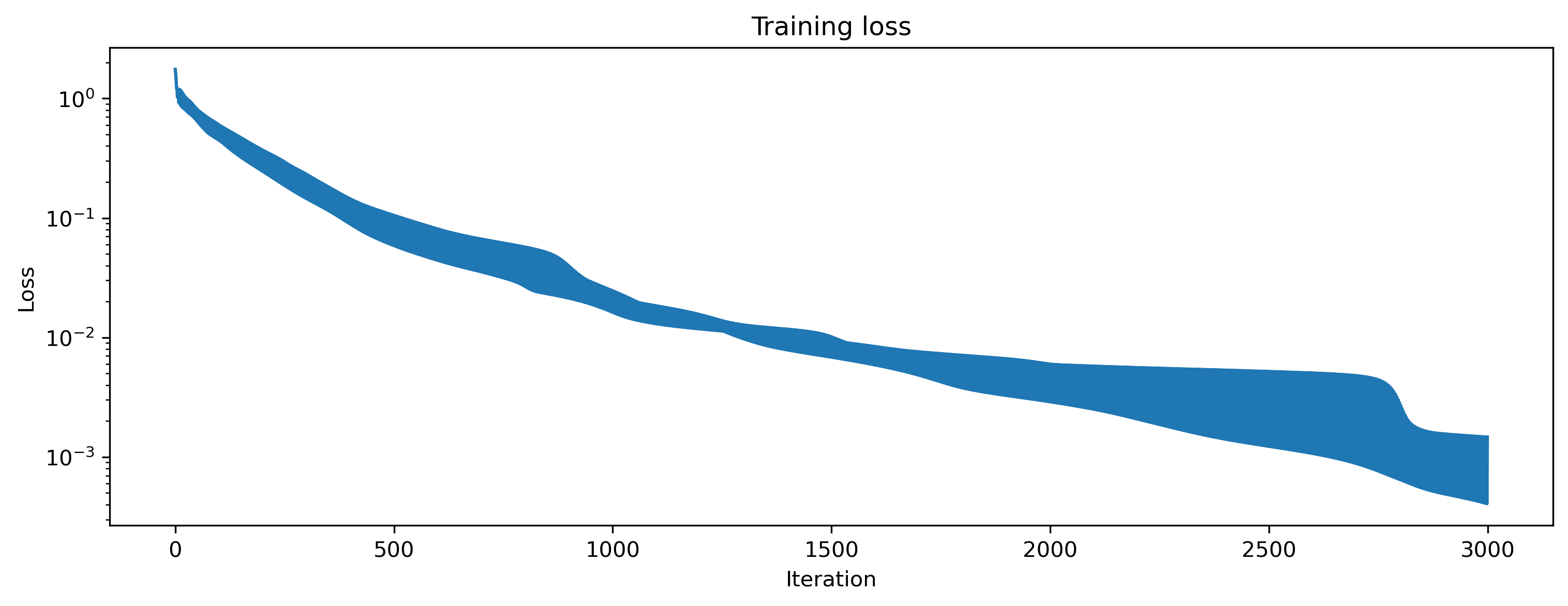
We can visualise the loss to see that we are indeed learning to match the desired network output.

# - Plot the loss over iterations
plt.plot(np.array(loss_t))
plt.yscale("log")
plt.xlabel("Iteration")
plt.ylabel("Loss")
plt.title("Training loss");

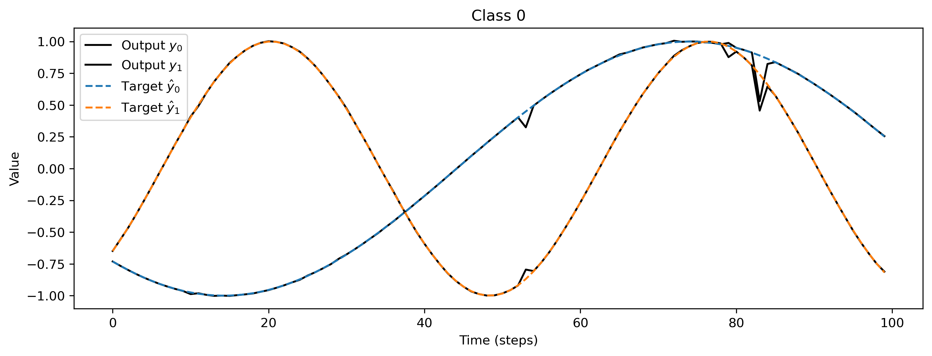
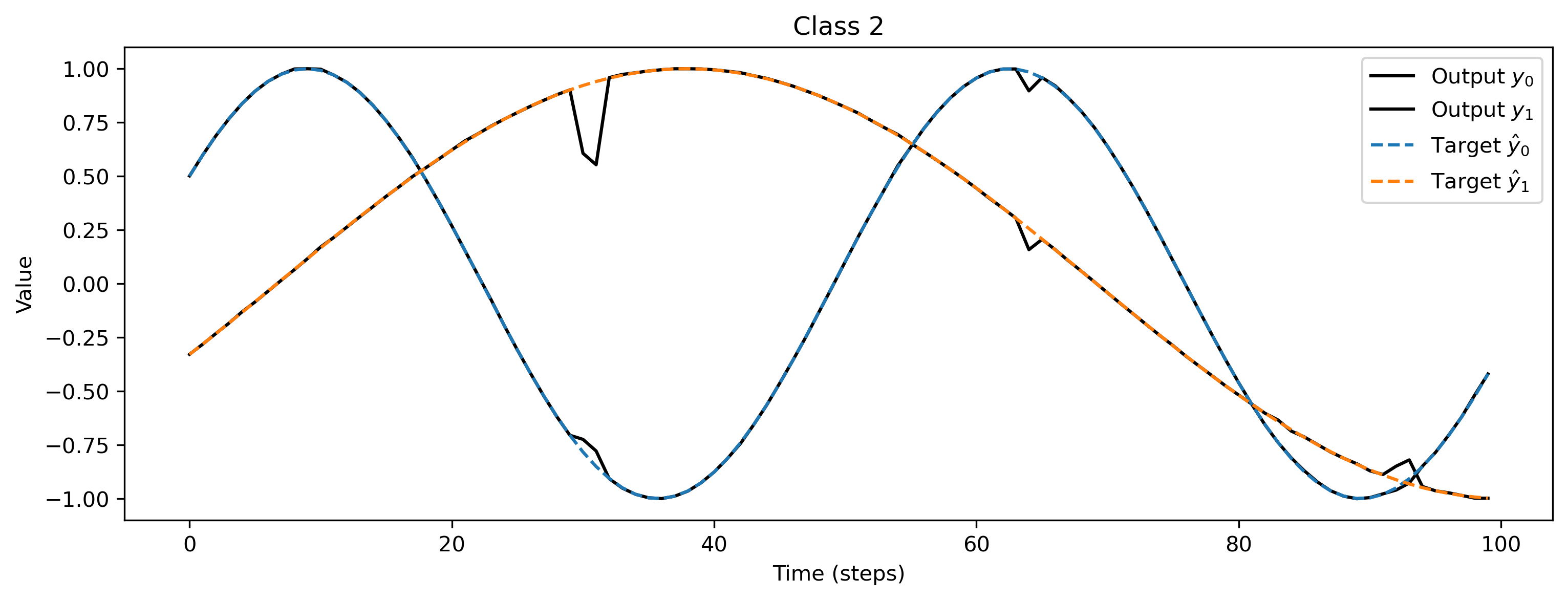
As a sanity check we can evaluate the network for each class, and plot the network output versus the target signals:

# - Apply the trained parameters to the network
params_hat = get_params(opt_state)
net = net.set_attributes(params_hat)

# - Evaluate classes
for i_class, sample in enumerate(ds):
    input, target = sample

    # - Evaluate network
    net = net.reset_state()
    output, _, _ = net(input, record=True)

    # - Plot output and target
    plt.figure()
    plt.plot(output[0], "k-")
    plt.plot(sample[1], "--")
    plt.xlabel("Time (steps)")
    plt.ylabel("Value")
    plt.legend(
        [
            "Output $y_0$",
            "Output $y_1$",
            "Target $\hat{y}_0$",
            "Target $\hat{y}_1$",
        ]
    )
    plt.title(f"Class {i_class}")

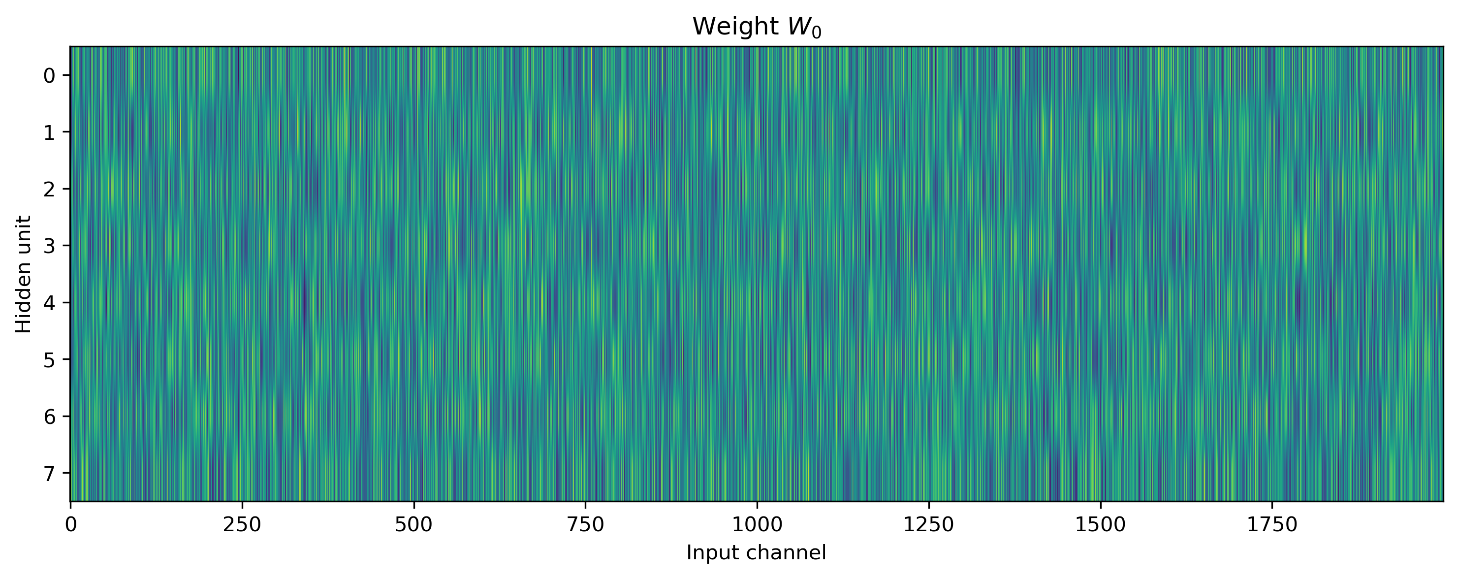
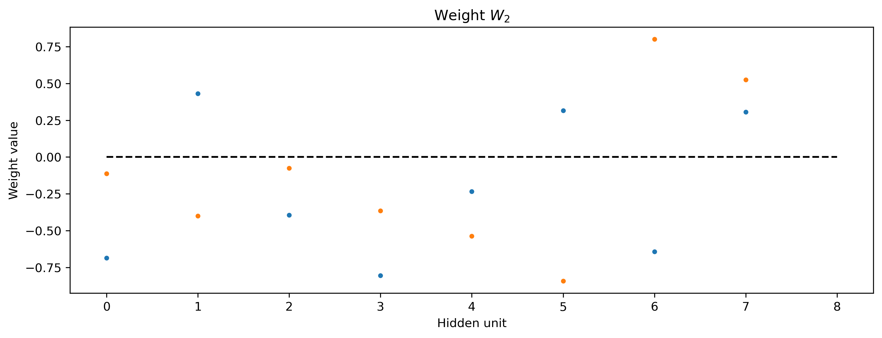
We can also visualise the network parameters directly, by indexing into the Sequential stack using standard Python indexing, and plotting the parameter attributes of interest.

# - Display network parameters
plt.figure()
plt.imshow(net[0].weight.T, aspect="auto")
plt.xlabel("Input channel")
plt.ylabel("Hidden unit")
plt.title("Weight $W_0$")

plt.figure()
plt.plot(net[2].weight, ".")
plt.plot([0, Nhidden], [0, 0], "k--")
plt.xlabel("Hidden unit")
plt.ylabel("Weight value")
plt.title("Weight $W_2$");

👩🏽‍🔬 Advanced Jax training topics

The Jax interface can of course be used just as conveniently on stateful Rockpool modules. However, the numerical stability of modules during evolution must be considered.

For example, the time constants of a neuron may not be negative, and if using a forward-Euler ODE solver, should be at least 10 times larger than the solver time-step \(\delta t\).

During optimisation, these constraints can easily be violated unless you take care to avoid it. In this example we show how you can include components in the loss function that enforce lower bounds on time constants. This can be extended to place bounds on any parameters.

Providing bounds on parameters during optimisation

We’ll illustrate this approach over a network including a stateful module nn.modules.RateEulerJax. This is a rate-based neuron with membrane leak, and can have an arbitrary transfer function. In this case, tanh is used.

# - Import the rate-based stateful module `RateEulerJax`
from rockpool.nn.modules import RateJax

# - Build a Jax network including a stateful module
Nhidden = 200
net_stateful = Sequential(
    LinearJax((Nin, Nhidden)),
    RateJax(Nhidden, activation_func="tanh"),
    LinearJax((Nhidden, Nout)),
)
print(net_stateful)

JaxSequential  with shape (2000, 2) {
    LinearJax '0_LinearJax' with shape (2000, 200)
    RateJax '1_RateJax' with shape (200,)
    LinearJax '2_LinearJax' with shape (200, 2)
}

To impose the bounds, we use the training utility module .training.jax_loss and the functions bounds_cost() and make_bounds().

bounds_cost() computes a cost penalty targetting parameter elements that violate a set of lower and/or upper bounds (greater-than and less-than constraint).

make_bounds() is a convenience function that returns pre-filled dictionaries to modify and pass to bounds_cost().

# - Import the convenience functions
from rockpool.training.jax_loss import bounds_cost, make_bounds

# - Generate a set of pre-configured bounds
lower_bounds, upper_bounds = make_bounds(net_stateful.parameters())
print("lower_bounds: ", lower_bounds, "upper_bounds: ", upper_bounds)

lower_bounds:
{
    '0_LinearJax': {'weight': -inf},
    '1_RateJax': {'bias': -inf, 'tau': -inf, 'threshold': -inf},
    '2_LinearJax': {'weight': -inf}
}
upper_bounds:
{
    '0_LinearJax': {'weight': inf},
    '1_RateJax': {'bias': inf, 'tau': inf, 'threshold': inf},
    '2_LinearJax': {'weight': inf}
}

By default these are initialised to \(\pm \infty\), indicating that no bounds should be imposed. We need to modify the lower bounds for the time constants, to make sure they do not fall below 10 ms.

# - Configure the bounds for this network
lower_bounds["1_RateJax"]["tau"] = 10e-3
print("lower_bounds: ", lower_bounds)

lower_bounds:
{
    '0_LinearJax': {'weight': -inf},
    '1_RateJax': {'bias': -inf, 'tau': 0.01, 'threshold': -inf},
    '2_LinearJax': {'weight': -inf}
}

Now we can include the bounds in a loss function, using the bounds_cost() function. The loss function below is an extended version of the simpler loss function in the previous example, which includes some parameter regularisation using l2sqr_norm() as well as the scaled bounds cost using bounds_cost().

def loss_mse_reg_bounds(parameters, net, inputs, target):
    # - Handle the network state — randomise or reset
    net = net.reset_state()

    # - Assign the provided parameters to the network
    net = net.set_attributes(parameters)

    # - Evolve the network to get the ouput
    output, _, _ = net(inputs)

    # - Compute a loss value w.r.t. the target output
    mse = l.mse(output, target)

    # - Add some parameter regularisation
    reg = l.l2sqr_norm(parameters) * 1e3

    # - Impose the bounds
    bounds = bounds_cost(parameters, lower_bounds, upper_bounds) * 1e3

    return mse + reg + bounds

We use a very similar training loop, which is essentially a copy of the previous example.

# - Initialise the optimiser with the initial parameters
params0 = deepcopy(net_stateful.parameters())
opt_state = init_fun(params0)

# - Get a compiled value-and-gradient function for the new loss
loss_vgf = jax.jit(jax.value_and_grad(loss_mse_reg_bounds))

# - Compile the optimiser update function
update_fun = jax.jit(update_fun)

# - Record the loss values over training iterations
loss_t = []
grad_t = []

num_epochs = 1000

# - Loop over iterations
i_trial = count()
for _ in tqdm(range(num_epochs)):
    for sample in ds:
        # - Get an input / target sample
        input, target = sample[0], sample[1]

        # - Get parameters for this iteration
        params = get_params(opt_state)

        # - Get the loss value and gradients for this iteration
        loss_val, grads = loss_vgf(params, net_stateful, input, target)

        # - Update the optimiser
        opt_state = update_fun(next(i_trial), grads, opt_state)

        # - Keep track of the loss
        loss_t.append(loss_val)

100%|██████████| 1000/1000 [00:23<00:00, 42.51it/s]

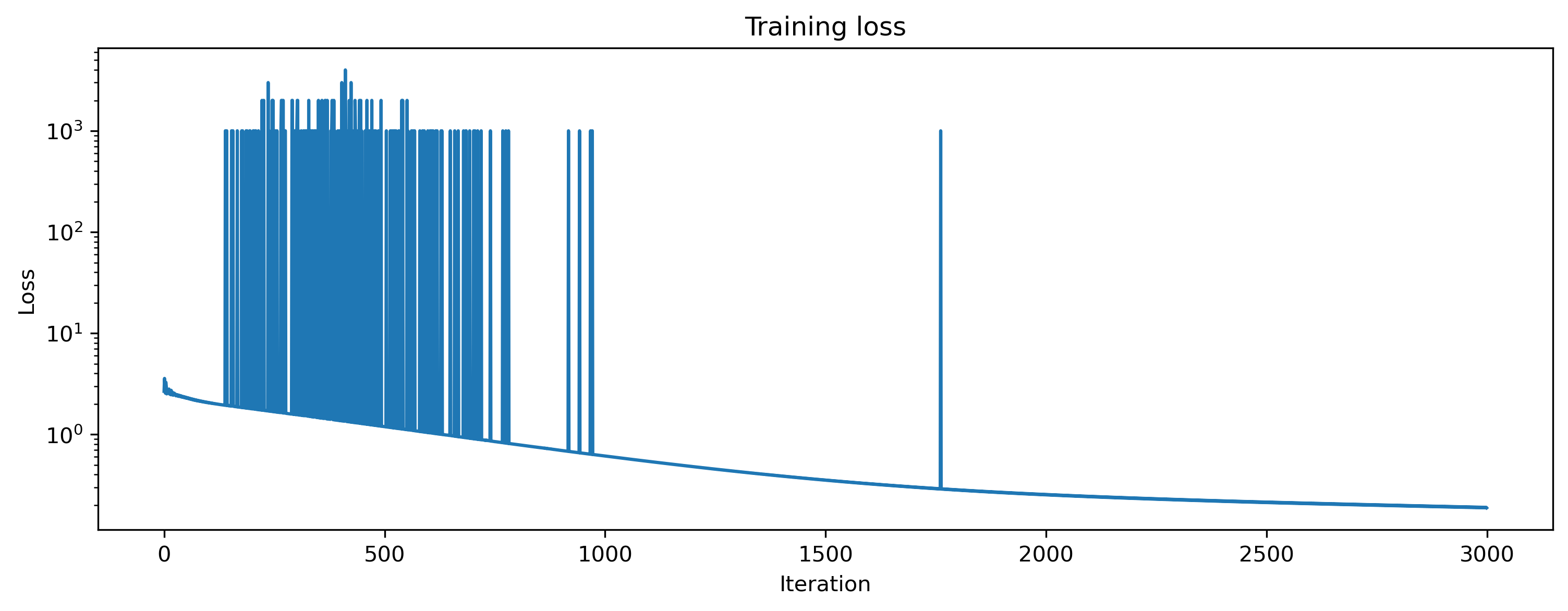
We can see from the loss values that the network is learning:

plt.plot(loss_t)
plt.yscale("log")
plt.xlabel("Iteration")
plt.ylabel("Loss")
plt.title("Training loss");

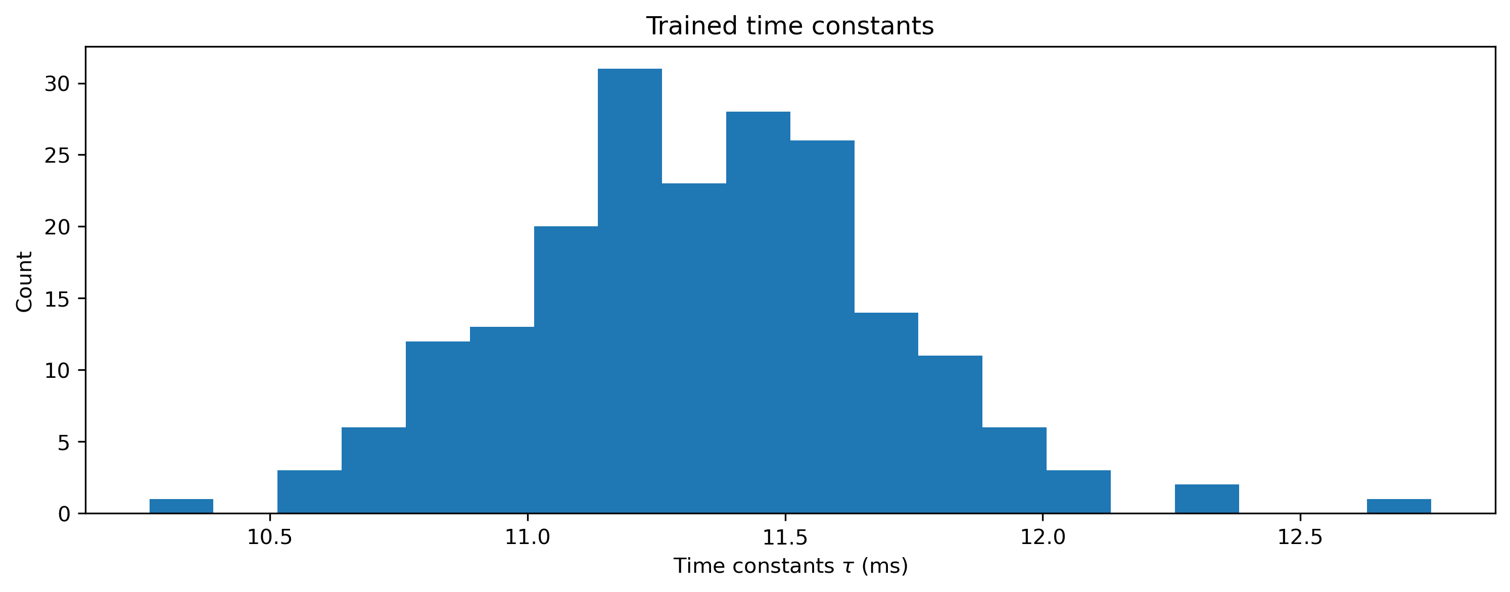
And if we visualise the time constants, we should see that none of them violate the lower bounds we imposed:

# - Get the final set of optimised parameters and apply them
params = get_params(opt_state)
net_stateful = net_stateful.set_attributes(params)

# - Visualise the time constants
plt.hist(net_stateful[1].tau * 1e3, 20)
plt.xlabel("Time constants $\\tau$ (ms)")
plt.ylabel("Count")
plt.title("Trained time constants");