This page was generated from docs/in-depth/howto-constrained-opt.ipynb. Interactive online version:

How To: Configure and perform constrained optimization in Rockpool

Spiking Neural Networks present a more complex optimisation problem than standard DNNs. This is due not only to the complex dynamics of spiking neurons but also to the additional classes of parameters present in SNNs.

DNNs usually optimise linear weights and bias parameters, all of which share a common scale and which can adopt unconstrained finite values. SNNs, on the other hand, contain various time-constant parameters of various formulations, which can only validly adopt a constrained range of values. For example, time constants in the form of synaptic and membrane \(\tau`s must be positive. Decay formulations for synapse and membrane time constants must range ``(0, 1)`\). Firing thresholds are usually also strictly positive values.

Because of this need, Rockpool provides convenient ways to access individual classes of parameters in a complex network via the Module.parameters() interface and a set of tools for easily configuring and imposing boundary constraints during optimisation.

This How To guide shows you how to use the training.torch_loss and training.jax_loss packages and the features of the utilities.tree_utils mini-library to set up constrained optimisation problems.

# - Make sure additional required packages are installed
import sys
!{sys.executable} -m pip install --quiet rich torch jax optax

from rich import print

import matplotlib.pyplot as plt
plt.rcParams['figure.figsize'] = [12, 4]
plt.rcParams['figure.dpi'] = 300

import numpy as np
import torch, jax, optax

[notice] A new release of pip available: 22.2.2 -> 23.0.1
[notice] To update, run: pip install --upgrade pip

/Users/Shared/anaconda3/envs/py38/lib/python3.8/site-packages/chex/_src/pytypes.py:37: FutureWarning: jax.tree_structure is deprecated, and will be removed in a future release. Use jax.tree_util.tree_structure instead.
  PyTreeDef = type(jax.tree_structure(None))

torch interface for constrained optimization

Rockpool supports both torch and jax optimisation backends, with a common API for setting up constrained optimisation. Here, we demonstrate the torch interface to set parameter constraints for a single LIF module.

# - Import the LIF module we will use
from rockpool.nn.modules import LIFTorch

# - Create a single LIF module
net = LIFTorch(1)
print('Module:', net)
print('Parameters:', net.parameters())

Module: LIFTorch  with shape (1, 1)

Parameters:
{
    'tau_mem': Parameter containing:
tensor([0.0200], requires_grad=True),
    'tau_syn': Parameter containing:
tensor([[0.0200]], requires_grad=True),
    'bias': Parameter containing:
tensor([0.], requires_grad=True),
    'threshold': Parameter containing:
tensor([1.], requires_grad=True)
}

Even this single spiking neuron has four parameters — two time constants for synapse and membrane (tau_syn and tau_mem), which must be positive; a bias parameter, which can adopt any value; and a threshold parameter which should also be positive.

Suppose either time constant becomes negative during training. In that case, the dynamics of the module will be undefined and most likely unstable, leading to a breakdown of both network dynamics and training.

Rockpool provides a cost function bounds_cost(), which imposes bounded parameter constraints. We also provide a helper function make_bounds(), which helps you build specifications for which parameters should be constrained and how.

Below we show how the cost function behaves as a parameter approaches and violates a constraint (0, 1).

# - Import the `make_bounds` and `bounds_cost` helper functions
from rockpool.training.torch_loss import make_bounds, bounds_cost

xs = np.linspace(-1, 2, 1001)
cost = [bounds_cost({'x': torch.tensor(x)}, {'x': 0.}, {'x': 1.}) for x in xs]

plt.figure()
plt.plot(xs, cost)
plt.plot([0, 0], [0, 3], 'r:')
plt.plot([1, 1], [0, 3], 'r:')
plt.xlabel('Parameter value')
plt.ylabel('Cost');

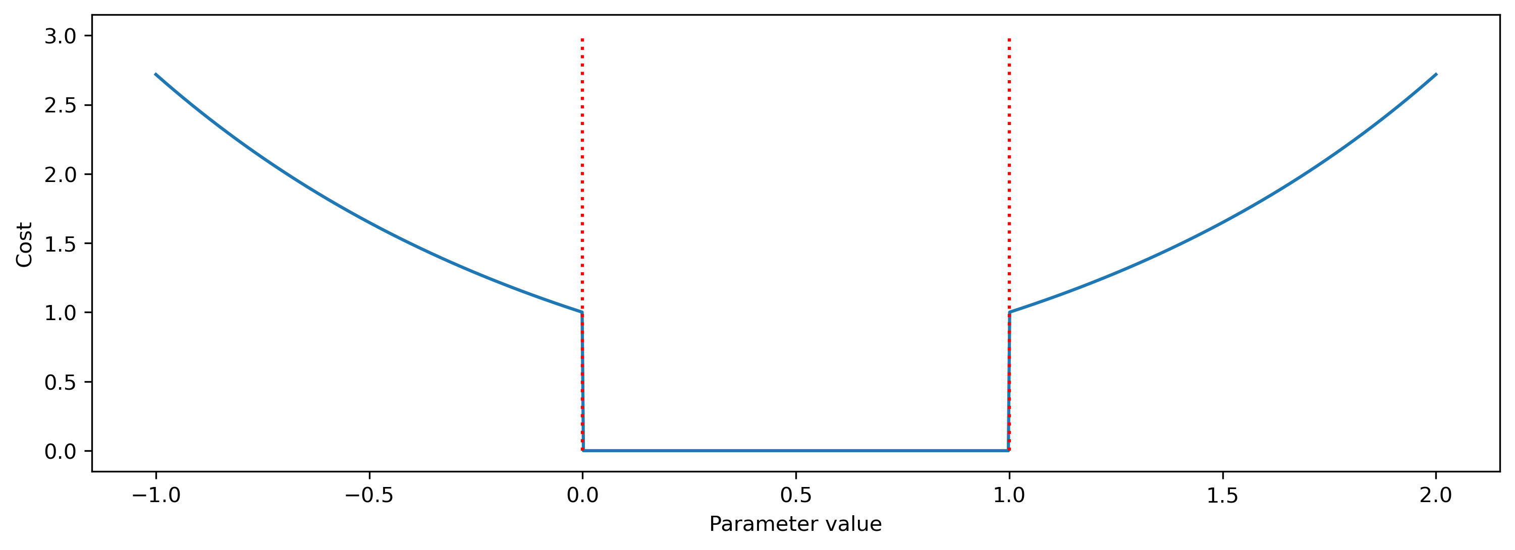
When no bounds are violated, the cost evaluates to zero. At the bounds, a cost of 1 is imposed, which increases for increasing violations.

Now let’s see how to create and apply bounds to the parameters of a LIF module.

The training.torch_loss.make_bounds() function takes the parameters of a Rockpool network and generates lower- and upper-bounds configuration dictionaries. These dictionaries mimic the structure of the network parameters.

# - Call `make_bounds` on the parameters of the module
lb, ub = make_bounds(net.parameters())
print(lb, ub)

{'tau_mem': -inf, 'tau_syn': -inf, 'bias': -inf, 'threshold': -inf}
{'tau_mem': inf, 'tau_syn': inf, 'bias': inf, 'threshold': inf}

By default, no parameters are constrained — the lower and upper bounds are set to negative and positive infinity, respectively. We set bounds by changing the values to finite lower and upper bounds. Let’s use (0ms, 200ms) as the constraints for tau_mem.

lb['tau_syn'] = 0.
ub['tau_syn'] = 200e-3
print(lb, ub)

{'tau_mem': -inf, 'tau_syn': 0.0, 'bias': -inf, 'threshold': -inf}
{'tau_mem': inf, 'tau_syn': 0.2, 'bias': inf, 'threshold': inf}

# - Evaluate the boundary constraint cost
print(bounds_cost(net.parameters(), lb, ub))

tensor(0., grad_fn=<SumBackward0>)

In this case, no bounds are violated, so the cost is zero.

Now let’s look at an example of a complex network with many layers and module nesting. We’ll define the network to use two different classes of leak parameters, needing different constraints on each class.

from rockpool.nn.modules import LinearTorch
from rockpool.nn.combinators import Sequential, Residual

net = Sequential(
    LinearTorch((2, 3)),
    LIFTorch(3, leak_mode="decays"),

    Residual(
        LinearTorch((3, 3)),
        LIFTorch(3, leak_mode="decays"),
    ),

    LinearTorch((3, 5)),
    LIFTorch(5, leak_mode="taus"),
)
print('Network:', net)
print('Parameters:', net.parameters())

Network: TorchSequential  with shape (2, 5) {
    LinearTorch '0_LinearTorch' with shape (2, 3)
    LIFTorch '1_LIFTorch' with shape (3, 3)
    TorchResidual '2_TorchResidual' with shape (3, 3) {
        LinearTorch '0_LinearTorch' with shape (3, 3)
        LIFTorch '1_LIFTorch' with shape (3, 3)
    }
    LinearTorch '3_LinearTorch' with shape (3, 5)
    LIFTorch '4_LIFTorch' with shape (5, 5)
}

Parameters:
{
    '0_LinearTorch': {
        'weight': Parameter containing:
tensor([[-1.7288,  0.3565,  0.7264],
        [-0.9882, -1.2147,  1.2812]], requires_grad=True)
    },
    '1_LIFTorch': {
        'alpha': Parameter containing:
tensor([0.5000, 0.5000, 0.5000], requires_grad=True),
        'beta': Parameter containing:
tensor([[0.5000],
        [0.5000],
        [0.5000]], requires_grad=True),
        'bias': Parameter containing:
tensor([0., 0., 0.], requires_grad=True),
        'threshold': Parameter containing:
tensor([1., 1., 1.], requires_grad=True)
    },
    '2_TorchResidual': {
        '0_LinearTorch': {
            'weight': Parameter containing:
tensor([[ 0.7141, -1.3781, -0.7695],
        [-0.8757, -0.6188, -0.4058],
        [-0.8914,  0.4774,  0.1480]], requires_grad=True)
        },
        '1_LIFTorch': {
            'alpha': Parameter containing:
tensor([0.5000, 0.5000, 0.5000], requires_grad=True),
            'beta': Parameter containing:
tensor([[0.5000],
        [0.5000],
        [0.5000]], requires_grad=True),
            'bias': Parameter containing:
tensor([0., 0., 0.], requires_grad=True),
            'threshold': Parameter containing:
tensor([1., 1., 1.], requires_grad=True)
        }
    },
    '3_LinearTorch': {
        'weight': Parameter containing:
tensor([[ 0.4936,  1.3029, -1.0018,  1.1015, -1.4031],
        [ 0.1428,  1.2207,  1.1742,  0.8693, -0.3616],
        [ 0.1114, -1.3645, -1.3504, -0.6766, -0.4882]], requires_grad=True)
    },
    '4_LIFTorch': {
        'tau_mem': Parameter containing:
tensor([0.0200, 0.0200, 0.0200, 0.0200, 0.0200], requires_grad=True),
        'tau_syn': Parameter containing:
tensor([[0.0200],
        [0.0200],
        [0.0200],
        [0.0200],
        [0.0200]], requires_grad=True),
        'bias': Parameter containing:
tensor([0., 0., 0., 0., 0.], requires_grad=True),
        'threshold': Parameter containing:
tensor([1., 1., 1., 1., 1.], requires_grad=True)
    }
}

This is a deeply nested network with a complex set of parameters. Luckily, Rockpool provides several convenient tools that make it easy to build constraints even for complex networks.

The Module.parameters() method allows you to easily extract families of parameters, helping you identify all time constants, for example. The Module.attributes_named() method allows you to specify particular named parameters.

The mini-library tree_utils helps you easily manipulate the parameter and constraint dictionaries to set chosen bounds. Here we’ll use the tree_utils.set_matching() function to set bounds for chosen parameter sets.

# - Import the tree utilities library
import rockpool.utilities.tree_utils as tu

# - Make template lower and upper bounds
lb, ub = make_bounds(net.parameters())

# - Set lower bounds on "decays" and "taus" family parameters
lb = tu.set_matching(lb, net.parameters('decays'), 0.5)
lb = tu.set_matching(lb, net.parameters('taus'), 0.)

# - Set upper bounds on "decays" family parameters
ub = tu.set_matching(ub, net.parameters('decays'), 1.)

# - Set an upper bound on a specific parameter name
ub = tu.set_matching(ub, net.attributes_named('tau_syn'), 500e-3)

print(lb, ub)

{
    '0_LinearTorch': {'weight': -inf},
    '1_LIFTorch': {'alpha': 0.5, 'beta': 0.5, 'bias': -inf, 'threshold': -inf},
    '2_TorchResidual': {
        '0_LinearTorch': {'weight': -inf},
        '1_LIFTorch': {'alpha': 0.5, 'beta': 0.5, 'bias': -inf, 'threshold': -inf}
    },
    '3_LinearTorch': {'weight': -inf},
    '4_LIFTorch': {'tau_mem': 0.0, 'tau_syn': 0.0, 'bias': -inf, 'threshold': -inf}
}
{
    '0_LinearTorch': {'weight': inf},
    '1_LIFTorch': {'alpha': 1.0, 'beta': 1.0, 'bias': inf, 'threshold': inf},
    '2_TorchResidual': {
        '0_LinearTorch': {'weight': inf},
        '1_LIFTorch': {'alpha': 1.0, 'beta': 1.0, 'bias': inf, 'threshold': inf}
    },
    '3_LinearTorch': {'weight': inf},
    '4_LIFTorch': {'tau_mem': inf, 'tau_syn': 0.5, 'bias': inf, 'threshold': inf}
}

# - Evaluate the boundary constraint cost for the full set of network parameters
print(bounds_cost(net.parameters(), lb, ub))

tensor(0., grad_fn=<SumBackward0>)

Defining and evaluating boundary losses for constrained optimisation is made simple, even for complex networks! Imposing the constraints is as simple as including torch_loss.bounds_cost() as a factor of the loss function during training, as in the example below.

from torch.optim import Adam
from torch.nn import CrossEntropyLoss

# - Initialise the optimiser
optimizer = Adam(net.parameters().astorch(), lr=1e-3)
func_loss = CrossEntropyLoss()

# - Dummy dataset
dataset = [(torch.tensor(np.random.rand(1, 1, 2), dtype=torch.float), torch.tensor(np.random.rand(1, 1, 5), dtype=torch.float))]

# - Optimiser loop over dataset
for input, target in dataset:
    optimizer.zero_grad()
    output, _, _ = net(input)

    # - Evaluate the functional and constraints losses
    loss = func_loss(output, target) + bounds_cost(net.parameters(), lb, ub)

    # - Perform the backward step
    loss.backward()
    optimizer.step()

jax interface for constrained optimization

The jax interface for constrained optimisation is identical to the torch interface. Here we demonstrate a similar constrained optimisation problem as above.

# - Import the Rockpool NN modules
from rockpool.nn.modules import LIFJax, LinearJax
from rockpool.nn.combinators import Sequential

# - Import tools from ``jax_loss`` instead of ``torch_loss``
from rockpool.training.jax_loss import make_bounds, bounds_cost

# - Import the tree utility package
from rockpool.utilities import tree_utils as tu

# - Set up a simple network
net = Sequential(
    LinearJax((2, 3)),
    LIFJax(3),
    LinearJax((3, 5)),
    LIFJax(5),
)
print('Network:', net)
print('Parameters:', net.parameters())

Network: JaxSequential  with shape (2, 5) {
    LinearJax '0_LinearJax' with shape (2, 3)
    LIFJax '1_LIFJax' with shape (3, 3)
    LinearJax '2_LinearJax' with shape (3, 5)
    LIFJax '3_LIFJax' with shape (5, 5)
}

Parameters:
{
    '0_LinearJax': {
        'weight': array([[ 1.45853284, -1.09957019, -0.31666267],
       [ 0.63834515,  1.47955107,  1.03358989]])
    },
    '1_LIFJax': {
        'tau_mem': DeviceArray([0.02, 0.02, 0.02], dtype=float32),
        'tau_syn': DeviceArray([[0.02],
             [0.02],
             [0.02]], dtype=float32),
        'bias': DeviceArray([0., 0., 0.], dtype=float32),
        'threshold': DeviceArray([1., 1., 1.], dtype=float32)
    },
    '2_LinearJax': {
        'weight': array([[ 0.3648217 ,  0.34105733,  1.23947428, -0.42756732,  0.6361447 ],
       [-0.19837451,  0.61290813,  1.25214626,  1.206278  ,  0.70346237],
       [ 0.73964399, -1.02753273, -0.28541291, -1.10618743,  0.78135608]])
    },
    '3_LIFJax': {
        'tau_mem': DeviceArray([0.02, 0.02, 0.02, 0.02, 0.02], dtype=float32),
        'tau_syn': DeviceArray([[0.02],
             [0.02],
             [0.02],
             [0.02],
             [0.02]], dtype=float32),
        'bias': DeviceArray([0., 0., 0., 0., 0.], dtype=float32),
        'threshold': DeviceArray([1., 1., 1., 1., 1.], dtype=float32)
    }
}

We again use training.jax_loss.make_bounds() to build a template configuration for constrained optimisation. We use the tree handling library and Module.parameters(), to set lower-bounds constraints on time constants.

# - Build a template configuration
lb, ub = make_bounds(net.parameters())
print(lb, ub)

{
    '0_LinearJax': {'weight': -inf},
    '1_LIFJax': {'bias': -inf, 'tau_mem': -inf, 'tau_syn': -inf, 'threshold': -inf},
    '2_LinearJax': {'weight': -inf},
    '3_LIFJax': {'bias': -inf, 'tau_mem': -inf, 'tau_syn': -inf, 'threshold': -inf}
}
{
    '0_LinearJax': {'weight': inf},
    '1_LIFJax': {'bias': inf, 'tau_mem': inf, 'tau_syn': inf, 'threshold': inf},
    '2_LinearJax': {'weight': inf},
    '3_LIFJax': {'bias': inf, 'tau_mem': inf, 'tau_syn': inf, 'threshold': inf}
}

# - Set lower bounds for time constants
lb = tu.set_matching(lb, net.parameters('taus'), 0.)
print(lb)

{
    '0_LinearJax': {'weight': -inf},
    '1_LIFJax': {'bias': -inf, 'tau_mem': 0.0, 'tau_syn': 0.0, 'threshold': -inf},
    '2_LinearJax': {'weight': -inf},
    '3_LIFJax': {'bias': -inf, 'tau_mem': 0.0, 'tau_syn': 0.0, 'threshold': -inf}
}

# - Evaluate the boundary constraint cost
print(bounds_cost(net.parameters(), lb, ub))

0.0

Therefore, the Rockpool-provided interface for setting bounds is almost identical between torch and jax. Below we show a very simple jax optimisation loop that incorporates the boundary constraints during optimisation.

# - Initialise the Adam optimiser with the initial network parameters
optimizer = optax.adam(1e-4)
params = net.parameters()
opt_state = optimizer.init(params)

# - Use an MSE loss
func_loss = lambda o, t: jax.numpy.mean((o - t) ** 2)

# - Network evaluation and loss function
def eval_loss(params, net, input, target):
    output, _, _ = net(input)
    loss = func_loss(output, target) + bounds_cost(params, lb, ub)

    return loss

# - Dummy dataset
dataset = [(np.random.rand(1, 1, 2), np.random.rand(1, 1, 5))]

# - Loop over dataset, evaluating loss and applying updates
for input, target in dataset:
    loss_value, grads = jax.value_and_grad(eval_loss)(params, net, input, target)
    updates, opt_state = optimizer.update(grads, opt_state, params)
    params = optax.apply_updates(params, updates)

Next steps

See 🏃🏽‍♀️ Training a Rockpool network with Jax for a jax training example that includes constraints.