This page was generated from docs/in-depth/torch-training.ipynb. Interactive online version:

👩🏼‍🚒 Training a Rockpool network with Torch

# - Switch off warnings
import warnings

warnings.filterwarnings("ignore")

# - Rich printing
try:
    from rich import print
except:
    pass

# - Import and configure matplotlib for plotting
import sys
!{sys.executable} -m pip install --quiet matplotlib
import matplotlib.pyplot as plt

%matplotlib inline
plt.rcParams["figure.figsize"] = [12, 4]
plt.rcParams["figure.dpi"] = 300

Considerations when using Torch

Torch is a very popular and easy to use machine learning library including a vast number of features. In Rockpool we want to make sure that our users have access to all the power provided by Torch in a nearly native way while also having access to the functionality provided by all other backends and Rockpool itself.

Torch can be used in two ways. First, an existing PyTorch model can be converted to work with the Rockpool API using the TorchModule.from_torch() function. Second, a model in Torch can be written in scratch using the TorchModule class. For details see: 🔥 Building Rockpool modules with Torch.

This notebook shows how to define a model using the TorchModule class and train it on a simple task. For comparibility, the used examples in this notebook are the same as in 🏃🏽‍♀️ Training a Rockpool network with Jax

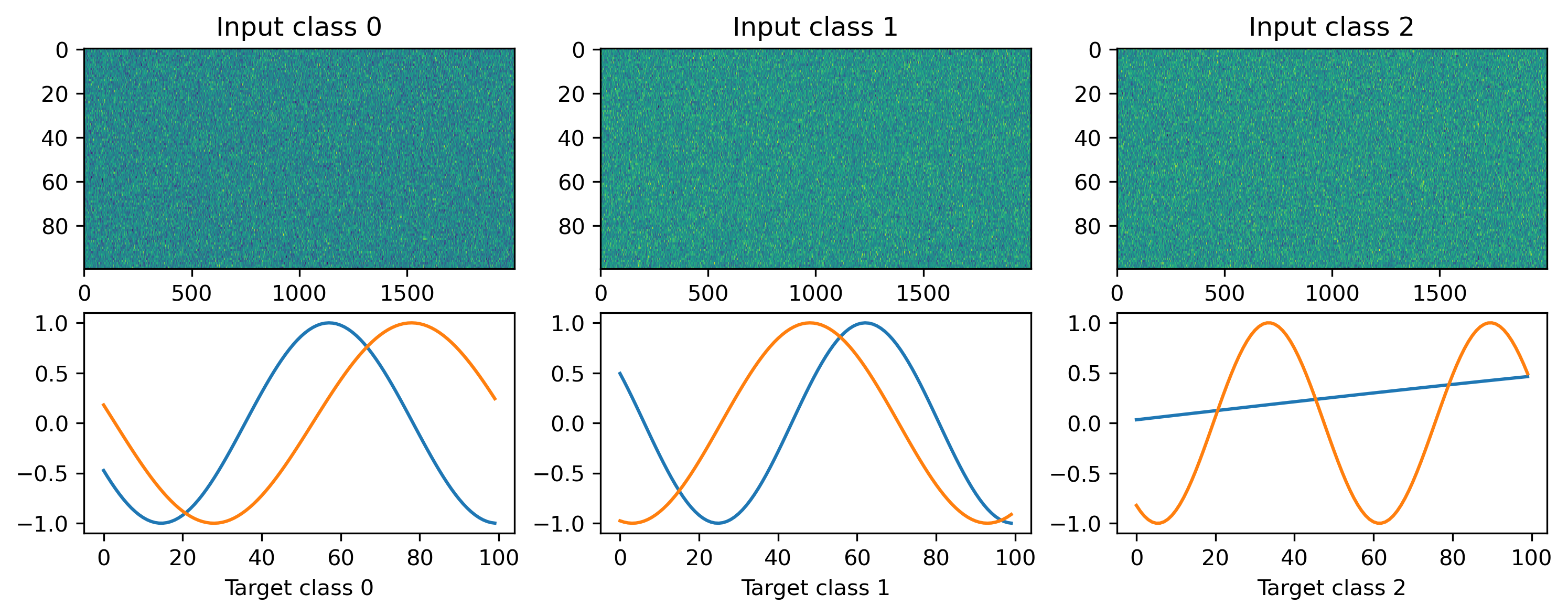
Define a task

We will define a simple random regression task, where random frozen input noise is mapped to randomly chosen smooth output signals. We implement this using a Dataset-compatible class, implementing the __len__() and __getitem__() methods.

import torch

# - Define a dataset class implementing the indexing interface
class MultiClassRandomSinMapping:
    def __init__(
        self,
        num_classes: int = 2,
        sample_length: int = 100,
        input_channels: int = 50,
        target_channels: int = 2,
    ):
        # - Record task parameters
        self._num_classes = num_classes
        self._sample_length = sample_length

        # - Draw random input signals
        self._inputs = torch.randn(num_classes, sample_length, input_channels) + 1.0

        # - Draw random sinusoidal target parameters
        self._target_phase = torch.rand(num_classes, 1, target_channels) * 2 * torch.pi
        self._target_omega = (
            torch.rand(num_classes, 1, target_channels) * sample_length / 50
        )

        # - Generate target output signals
        time_base = torch.atleast_2d(torch.arange(sample_length) / sample_length).T
        self._targets = torch.sin(
            2 * torch.pi * self._target_omega * time_base + self._target_phase
        )

    def __len__(self):
        # - Return the total size of this dataset
        return self._num_classes

    def __getitem__(self, i):
        # - Return the indexed dataset sample
        return torch.Tensor(self._inputs[i]), torch.Tensor(self._targets[i])

# - Instantiate a dataset
Nin = 2000
Nout = 2
num_classes = 3
T = 100
ds = MultiClassRandomSinMapping(
    num_classes=num_classes,
    input_channels=Nin,
    target_channels=Nout,
    sample_length=T,
)

# Display the dataset classes
plt.figure()
for i, sample in enumerate(ds):
    plt.subplot(2, len(ds), i + 1)
    plt.imshow(sample[0], aspect='auto', interpolation='none')
    plt.title(f"Input class {i}")

    plt.subplot(2, len(ds), i + len(ds) + 1)
    plt.plot(sample[1])
    plt.xlabel(f"Target class {i}")

Defining a network

We’ll define a very simple MLP-like network to solve the regression task we just defined. In this simple network we define one hidden layer with a tanh non-linearity.

from rockpool.nn.modules import LinearTorch, InstantTorch
from rockpool.nn.combinators import Sequential


def SimpleNet(Nin, Nhidden, Nout):
    return Sequential(
        LinearTorch((Nin, Nhidden)),
        InstantTorch((Nhidden,), torch.tanh),
        LinearTorch((Nhidden, Nout)),
    )

Nhidden = 10
net = SimpleNet(Nin, Nhidden, Nout)

Training loop

As usually done for a regression task, we are using the MSE loss and Adam during training. The whole workflow is very similar to the native Torch API. The one difference to the standard Torch API is that the forward function returns a tuple of (output, state, recordings).

# - Useful imports
from tqdm.autonotebook import tqdm
from torch.optim import Adam, SGD
from torch.nn import MSELoss

# - Get the optimiser functions
optimizer = Adam(net.parameters().astorch(), lr=1e-4)

# - Loss function
loss_fun = MSELoss()

# - Record the loss values over training iterations
loss_t = []

num_epochs = 3000

# - Loop over iterations
for _ in tqdm(range(num_epochs)):
    for input, target in ds:

        optimizer.zero_grad()

        output, state, recordings = net(input)

        loss = loss_fun(output, target)
        loss.backward()
        optimizer.step()

        # - Keep track of the loss
        loss_t.append(loss.item())

100%|██████████| 3000/3000 [00:36<00:00, 82.82it/s]

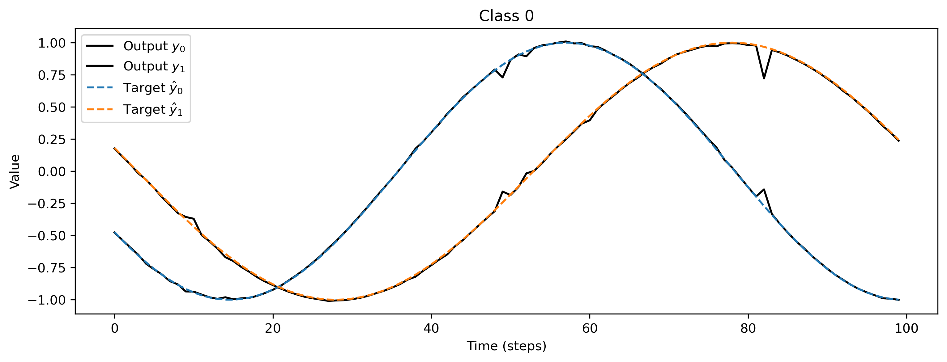
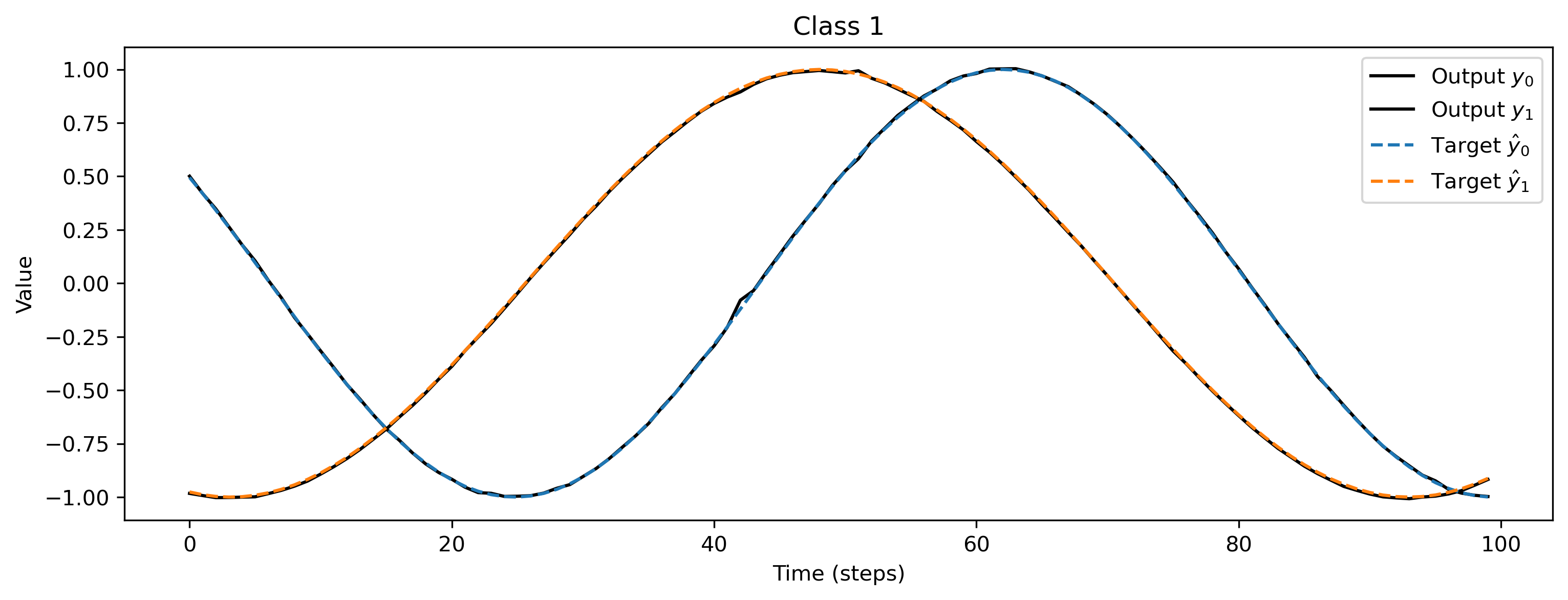
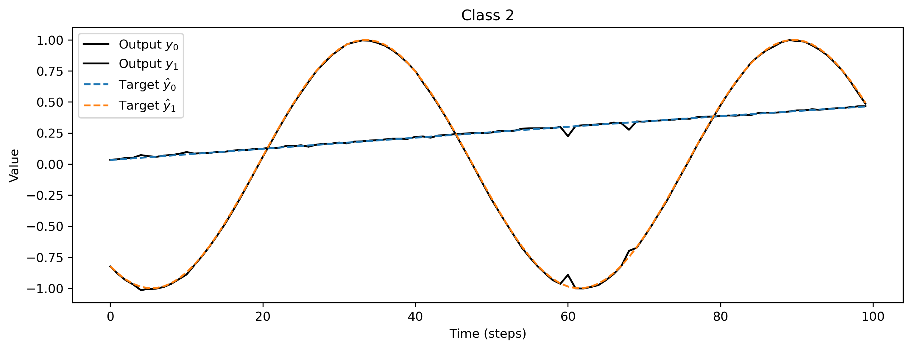
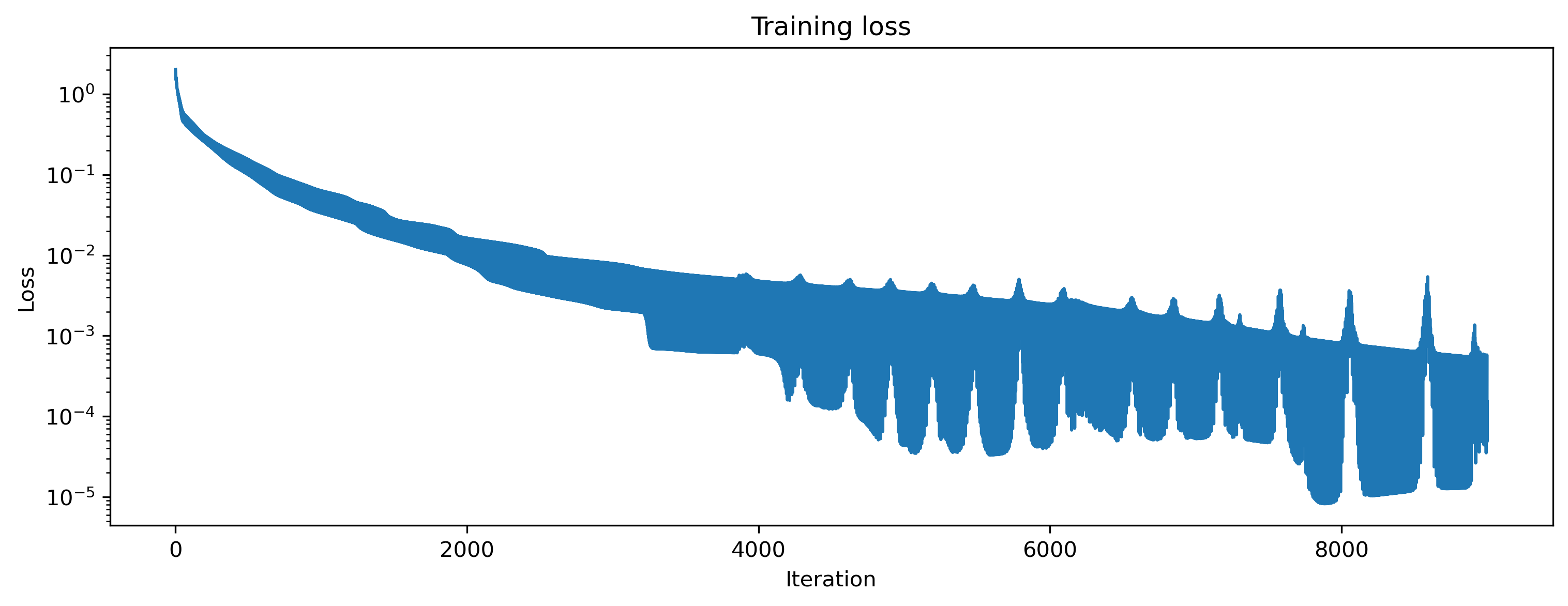
After training, we inspect the loss and plot the result of the training. We can see that the loss is decreasing and the predicted curves match the target curves nicely.

# - Plot the loss over iterations
plt.plot(loss_t)
plt.yscale("log")
plt.xlabel("Iteration")
plt.ylabel("Loss")
plt.title("Training loss");

# - Evaluate classes
for i_class, [input, target] in enumerate(ds):

    # - Evaluate network
    net = net.reset_state()
    output, _, _ = net(input, record=True)

    # - Plot output and target
    plt.figure()
    plt.plot(output[0].detach().cpu().numpy(), "k-")
    plt.plot(target, "--")
    plt.xlabel("Time (steps)")
    plt.ylabel("Value")
    plt.legend(
        [
            "Output $y_0$",
            "Output $y_1$",
            "Target $\hat{y}_0$",
            "Target $\hat{y}_1$",
        ]
    )
    plt.title(f"Class {i_class}")