This page was generated from docs/in-depth/api-high-level.ipynb. Interactive online version:

⏱ High-level TimedModule API

The high-level API in Rockpool allows you to build networks of stateful neurons that accept and manipulate time-series data natively.

Time-series data in Rockpool is encapsulated by TimeSeries classes: TSContinuous for continuous signals, and TSEvent for discrete events (see Working with time series data for an overview).

The TimedModule API allows you to specify modules that receive TimeSeries objects as input; process them; and return TimeSeries objects as output.

Constructing a TimedModule

Instantiating a TimedModule works in a very similar way to the low-level API. You must specify the simulation time-step dt, if a useful default is not provided. TimedModule will try to set a sensible dt internally if it can, but you usually want to have control over this.

# - Switch off warnings
import warnings
warnings.filterwarnings('ignore')

# - Useful imports
import numpy as np

try:
    from rich import print
except:
    pass

from rockpool.nn.combinators import Sequential
from rockpool.nn.modules import Rate, Linear

# - Construct the TimedModule
Nin = 1
Nout = 5
dt = 1e-3
tmod = Sequential(Linear((Nin, Nout)), Rate(Nout)).timed(dt = dt)
print(tmod)

TimedModuleWrapper  with shape (1, 5) {
    ModSequential '_module' with shape (1, 5) {
        Linear '0_Linear' with shape (1, 5)
        Rate '1_Rate' with shape (5,)
    }
} with ModSequential '_module' as module

Evolving a TimedModule

Passing time series data through a TimedModule is very convenient. A TimedModule knows how to handle TimeSeries objects natively, and handles any required sampling, resampling, rasterisation etc. internally.

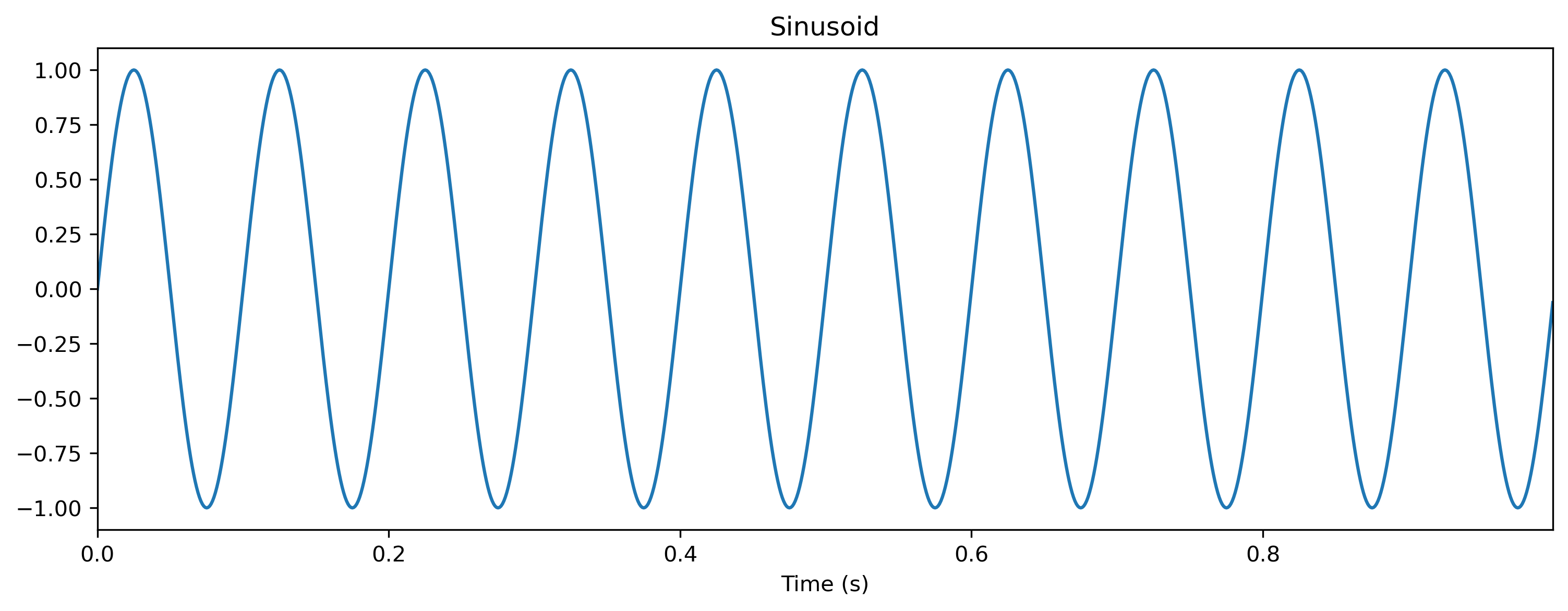
Let’s start by defining a sinusoid waveform to use as input.

# - Import time-series handling classes
from rockpool import TSContinuous

# - Import and configure matplotlib for plotting
import sys
!{sys.executable} -m pip install --quiet matplotlib
import matplotlib.pyplot as plt
%matplotlib inline
plt.rcParams['figure.figsize'] = [12, 4]
plt.rcParams['figure.dpi'] = 300

# - Create a sinusoidal input signal
T = 1000
omega = 10
time_base = np.arange(T) * dt
ts_sin = TSContinuous.from_clocked(
    np.sin(time_base * 2 * np.pi * omega),
    dt = dt,
    periodic = True,
    name = 'Sinusoid',
)
ts_sin.plot();

Now we can evolve the TimedModule by simply calling it with the input time series. The evolve() arguments are slightly different to that for the low-level API:

output_ts, new_state, recorded_state = evolve(ts_input: TimeSeries, duration: float, num_timesteps: int)

You can specify the evolution duration either explicity in terms of real time (duration in seconds), or in units of dt (num_timesteps); or implicitly by simply providing the input signal ts_input.

If you just provide ts_input, then Rockpool will evolve the TimedModule for the remaining valid duration of time series. Remember that Rockpool

# - Evolve the TimedModule
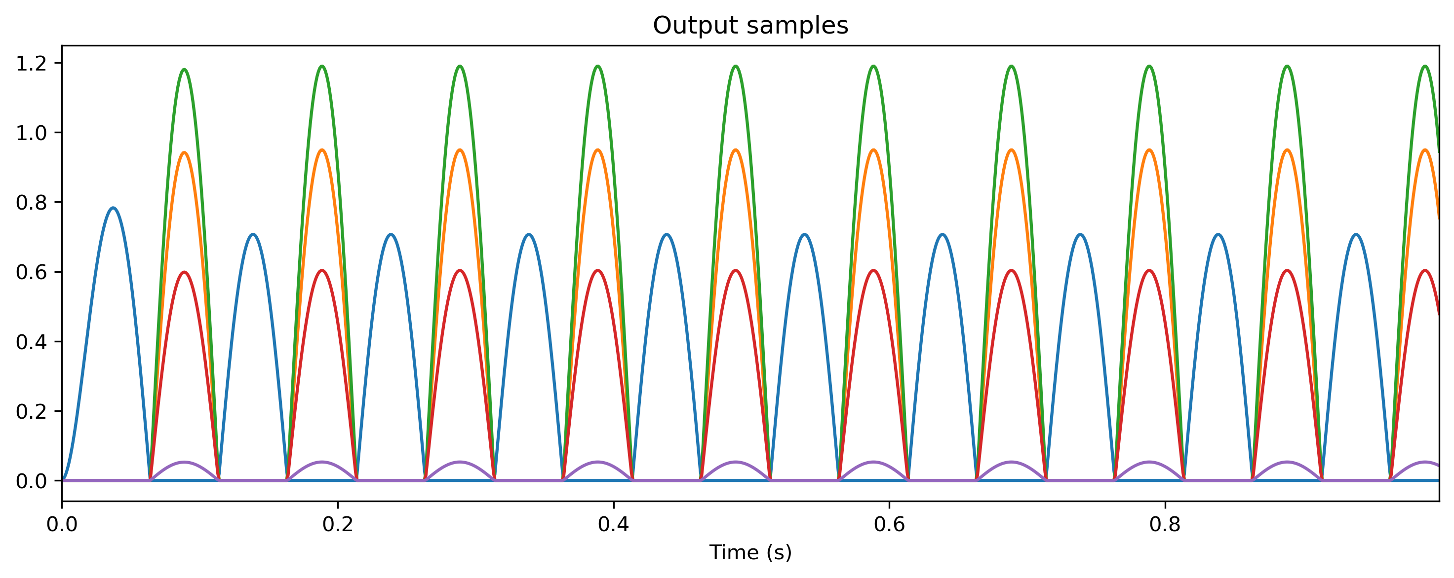
output_ts, _, _ = tmod(ts_sin)
plt.figure();
print(output_ts);
output_ts.plot();

non-periodic TSContinuous object `Output samples` from t=0.0 to 1.0. Samples: 1000. Channels: 5

Inspecting a TimedModule

Inspecting a TimedModule uses the common Rockpool API. All attributes can be accessed using standard Python “dot” indexing notation, or the module can be inspected using the parameters(), state(), simulation_parameters() and modules() methods.

# - Examine the parameters
print('Parameters:', tmod.parameters())

# - Examine the state
print('State:', tmod.state())

# - Examine the simulation parameters
print('Simulation parameters:', tmod.simulation_parameters())

# - `TimedModules` also have time
print('Time:', tmod.t)

Parameters:
{
    '_module': {
        '0_Linear': {'weight': array([[ 1.1175366 , -1.50156676, -1.88202227, -0.95408104, -0.08374108]])},
        '1_Rate': {
            'tau': array([0.02, 0.02, 0.02, 0.02, 0.02]),
            'bias': array([0., 0., 0., 0., 0.]),
            'threshold': array([0., 0., 0., 0., 0.])
        }
    }
}

State:
{
    '_module': {
        '0_Linear': {},
        '1_Rate': {'x': array([-0.56143606,  0.75436789,  0.94550386,  0.47931808,  0.04207044])}
    }
}

Simulation parameters:
{
    'dt': 0.001,
    '_module': {
        'dt': 0.001,
        '0_Linear': {},
        '1_Rate': {'dt': 0.001, 'noise_std': 0.0, 'act_fn': <function H_ReLU at 0x7f05e46a4ee0>}
    }
}

Time: 1.0

Building a network using nested TimedModule s

You can inherit from the TimedModule base class to build arbitrary networks, combining other TimedModule s as you like. TimedModule takes care of many things for you, including all the handling of TimeSeries data.

You can keep all data in TimeSeries objects and maniupulate the data in that format, using the operator support from TimeSeries subclases. Alternatively you can use convenience methods provided by TimedModule to assist with converting signals to and from TimeSeries objects.

To define a network as a TimedModule subclass, you need to minimally define an __init__() method and an evolve() method.

The __init__() method specifies and initialises parameters for your network, and initialises any required submodules. The submodules take care of specifying and initialise their own parameters and state.

In the example below, we build a small feed-forward network as a TimedModule, with one layer of linear input weights and two additional layers of ReLU rate units with weighting in-between. We show how to maintain all signals as TimeSeries objects through evolution. To do so, all submodules must themselves be TimedModule subclasses.

# - Import the base class and a TimedModule to use as a submodule
from rockpool.nn.modules import TimedModule, Rate
from rockpool.parameters import Parameter
from rockpool import TimeSeries

# - Define a new TimedModule
class ffwd_tmod_net(TimedModule):
    # - Provide an `__init__` method to specify required parameters and modules
    #   Here you check, define and initialise whatever parameters and
    #   state you need for your module.
    def __init__(self,
                 shape,
                 dt = 1.,
                 *args,
                 **kwargs,
                ):
        # - Call superclass initialisation
        #   This is always required for a `Module` class
        super().__init__(shape = shape, dt = dt, *args, **kwargs)

        # - Specify weights attributes
        #   We need a weights matrix for our input weights.
        #   We specify the shape explicitly, and provide an initialisation function.
        #   We also specify a family for the parameter, "weights". This is used to
        #   query parameters conveniently, and is a good idea to provide.
        self.w_0 = Parameter(
            shape = self.shape[0:2],
            init_func = lambda s: np.zeros(s),
            family = 'weights',
        )

        self.w_1 = Parameter(
            shape = self.shape[1:3],
            init_func = lambda s: np.zeros(s),
            family = 'weights',
        )

        self.w_2 = Parameter(
            shape = self.shape[2:4],
            init_func = lambda s: np.zeros(s),
            family = 'weights',
        )

        # - Specify and add submodules
        #   These will be the neurons in our layer, to receive the weighted
        #   input signals. This sub-module will be automatically configured
        #   internally, to specify the required state and parameters
        self.neurons1 = Rate(self.shape[1], dt = dt).timed()
        self.neurons2 = Rate(self.shape[2], dt = dt).timed()

    # - The `evolve` method contains the internal logic of your module
    #   `evolve` takes care of passing data in and out of the module,
    #   and between sub-modules if present.
    def evolve(self,
               ts_input: TimeSeries,
               duration: float,
               num_timesteps: int,
               record: bool = False,
               *args, **kwargs):
        # - Pass input data through the input weights
        x = ts_input @ self.w_0

        # - Pass the signals through the neurons and hidden weights
        x, _, _ = self.neurons1(x)
        x = x @ self.w_1
        x, _, _ = self.neurons2(x)
        x = x @ self.w_2

        # - Return the module output
        return x, {}, {}

Nin = 3
Nout = 1
dt = 1

tmod = ffwd_tmod_net((Nin, 5, 7, Nout), dt = dt)
print(tmod)

ffwd_tmod_net  with shape (3, 5, 7, 1) {
    TimedModuleWrapper 'neurons1' with shape (5, 5) {
        Rate '_module' with shape (5,)
    }
    TimedModuleWrapper 'neurons2' with shape (7, 7) {
        Rate '_module' with shape (7,)
    }
}

# - Examine the nested parameters of the TimedModule
print(tmod.parameters())

{
    'w_0': array([[0., 0., 0., 0., 0.],
       [0., 0., 0., 0., 0.],
       [0., 0., 0., 0., 0.]]),
    'w_1': array([[0., 0., 0., 0., 0., 0., 0.],
       [0., 0., 0., 0., 0., 0., 0.],
       [0., 0., 0., 0., 0., 0., 0.],
       [0., 0., 0., 0., 0., 0., 0.],
       [0., 0., 0., 0., 0., 0., 0.]]),
    'w_2': array([[0.],
       [0.],
       [0.],
       [0.],
       [0.],
       [0.],
       [0.]]),
    'neurons1': {
        '_module': {
            'tau': array([0.02, 0.02, 0.02, 0.02, 0.02]),
            'bias': array([0., 0., 0., 0., 0.]),
            'threshold': array([0., 0., 0., 0., 0.])
        }
    },
    'neurons2': {
        '_module': {
            'tau': array([0.02, 0.02, 0.02, 0.02, 0.02, 0.02, 0.02]),
            'bias': array([0., 0., 0., 0., 0., 0., 0.]),
            'threshold': array([0., 0., 0., 0., 0., 0., 0.])
        }
    }
}

# - Set the weights to something non-zero
p = tmod.parameters()
p['w_0'] = np.random.normal(size = p['w_0'].shape) + 1
p['w_1'] = np.random.normal(size = p['w_1'].shape) + 1
p['w_2'] = np.random.normal(size = p['w_2'].shape) + 1

# - Assign the new parameters
tmod.set_attributes(p)
print('Weights:', tmod.parameters())

Weights:
{
    'w_0': array([[ 1.73722151,  1.30356212,  0.55156482,  2.8019148 ,  1.09027286],
       [ 1.97210989,  1.88721147,  1.29312512, -0.28583698,  1.45047169],
       [ 0.04967296, -0.94915265,  1.37862991,  1.29235999,  0.050853  ]]),
    'w_1': array([[ 1.52490803,  0.53006083,  3.11873417, -0.15332358,  1.51820289,
         2.88070423, -0.55447475],
       [ 0.03845312,  0.76734798,  0.77595556,  2.23176957, -0.90711186,
         1.39216172,  0.132243  ],
       [ 0.47959018,  0.99225231,  0.54699617,  0.91157126,  0.61972611,
         3.7774115 ,  2.23284232],
       [ 0.56585036,  2.65117266,  0.4449058 ,  0.0736041 ,  0.02211706,
        -0.34763718, -0.79899013],
       [ 1.51294292,  0.81017138,  1.07416865, -1.13288234,  0.92521921,
         1.6997927 ,  1.38329005]]),
    'w_2': array([[-0.01196603],
       [ 1.74152837],
       [-0.35683857],
       [-0.29947419],
       [ 0.38918974],
       [ 1.76011316],
       [ 0.96554928]]),
    'neurons1': {
        '_module': {
            'tau': array([0.02, 0.02, 0.02, 0.02, 0.02]),
            'bias': array([0., 0., 0., 0., 0.]),
            'threshold': array([0., 0., 0., 0., 0.])
        }
    },
    'neurons2': {
        '_module': {
            'tau': array([0.02, 0.02, 0.02, 0.02, 0.02, 0.02, 0.02]),
            'bias': array([0., 0., 0., 0., 0., 0., 0.]),
            'threshold': array([0., 0., 0., 0., 0., 0., 0.])
        }
    }
}

# - Generate some white noise input
ts_input = TSContinuous.from_clocked(np.random.rand(1000, Nin),
                                     name = 'White noise',
                                     dt = dt, periodic = True,
                                    )
print('Input:', ts_input)
ts_input.plot()

# - Evolve the TimedModule with the input
ts_output, _, rec = tmod(ts_input)

# - Display the output
print('Output:', ts_output)
plt.figure()
ts_output.plot();

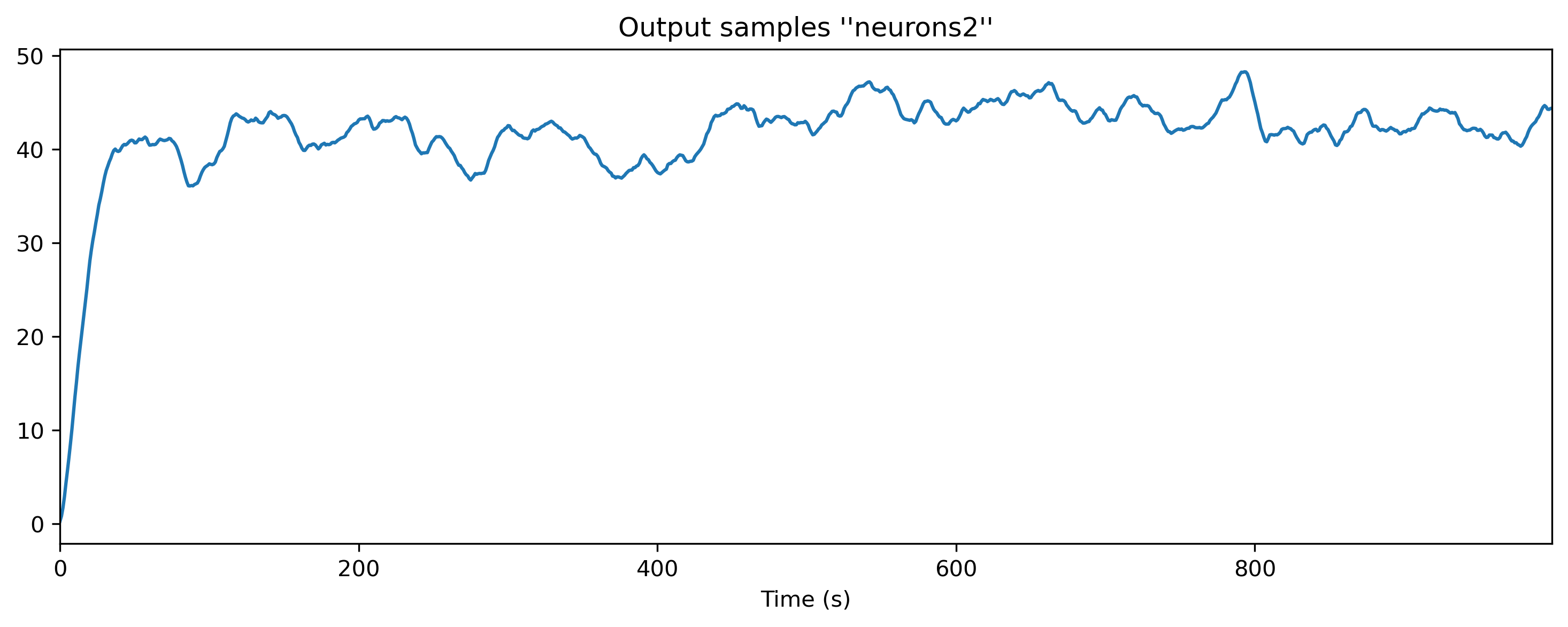
Input: periodic TSContinuous object `White noise` from t=0.0 to 1000.0. Samples: 1000. Channels: 3

Output: non-periodic TSContinuous object `Output samples ''neurons2''` from t=0.0 to 1000.0. Samples: 1000.
Channels: 1

Building a network using internal Module s

Sometimes the modules you want to use to build a network are not available as TimedModule s. In this case you can use the low-level Module API internally, and still present a high-level TimedModule API interface to the outside world.

To do so, TimedModule provides a number of convenience methods for wrapping, unwrapping and rasterising time series data:

time_base, input_raster, num_timesteps = self._repare_input(
    ts_input: TimeSeries,
    duration: float,
    num_timesteps: int
)

ts_output = self._gen_timeseries(output_raster, **kwargs)

The example below illustrates how to use these methods to build a similar network architecture to the one above, but using low-level Module API submodules.

# - Import the base class and a Module to use as a submodule
from rockpool.nn.modules import TimedModule
from rockpool.parameters import Parameter
from rockpool.nn.modules import RateJax
from rockpool import TimeSeries

# - Define a new TimedModule
class ffwd_tmod_net2(TimedModule):
    # - Provide an `__init__` method to specify required parameters and modules
    #   Here you check, define and initialise whatever parameters and
    #   state you need for your module.
    def __init__(self,
                 shape,
                 *args,
                 **kwargs,
                ):
        # - Call superclass initialisation
        #   This is always required for a `Module` class
        super().__init__(shape = shape, *args, **kwargs)

        # - Specify weights attributes
        #   We need weights matrices for our layer weights.
        #   We specify the shapes explicitly, and provide an initialisation function.
        #   We also specify a family for the parameter, "weights". This is used to
        #   query parameters conveniently, and is a good idea to provide.
        self.w0 = Parameter(shape = self.shape[0:2],
                            init_func = lambda s: np.zeros(s),
                            family = 'weights',
                            )

        self.w1 = Parameter(shape = self.shape[1:3],
                            init_func = lambda s: np.zeros(s),
                            family = 'weights',
                            )

        # - Specify and add submodules
        #   These will be the neurons in our layer, to receive the weighted
        #   input signals. These sub-modules will be automatically configured
        #   internally, to specify the required state and parameters
        self.neurons0 = RateJax(self.shape[1])
        self.neurons1 = RateJax(self.shape[2])

    # - The `evolve` method contains the internal logic of your module
    #   `evolve` takes care of passing data in and out of the module,
    #   and between sub-modules if present.
    def evolve(self,
               ts_input: TimeSeries,
               duration: float,
               num_timesteps: int,
               record: bool = False,
               *args, **kwargs):
        # - First we need to rasterise the input time series.
        #   We can use the convenience method `_prepare_input()` for this
        time_base, input_raster, num_timesteps = self._prepare_input(
            ts_input, duration, num_timesteps
        )

        # - Pass input data through the input weights
        x0 = input_raster @ self.w0

        # - Pass the signals through the neurons
        x1, _, _ = self.neurons0(x0)

        # - Second layer weights
        x2 = x1 @ self.w1

        # - Second layer neurons
        x3, _, _ = self.neurons1(x2)

        # - We need to re-wrap the output raster as a TimeSeries object
        #   To do this we can use the convenience method `_gen_timeseries()`
        output_ts = self._gen_timeseries(x3)

        # - Return the module output
        return output_ts, {}, {}

# - Instantiate the module
tmod = ffwd_tmod_net2((Nin, 5, 7, Nout), dt = dt)
print(tmod)

ffwd_tmod_net2  with shape (3, 5, 7, 1) {
    RateJax 'neurons0' with shape (5,)
    RateJax 'neurons1' with shape (7,)
}

print('Input:', ts_input)
ts_input.plot()

# - Evolve the TimedModule with the input
ts_output, _, rec = tmod(ts_input)

# - Display the output
print('Output:', ts_output)
plt.figure()
ts_output.plot();

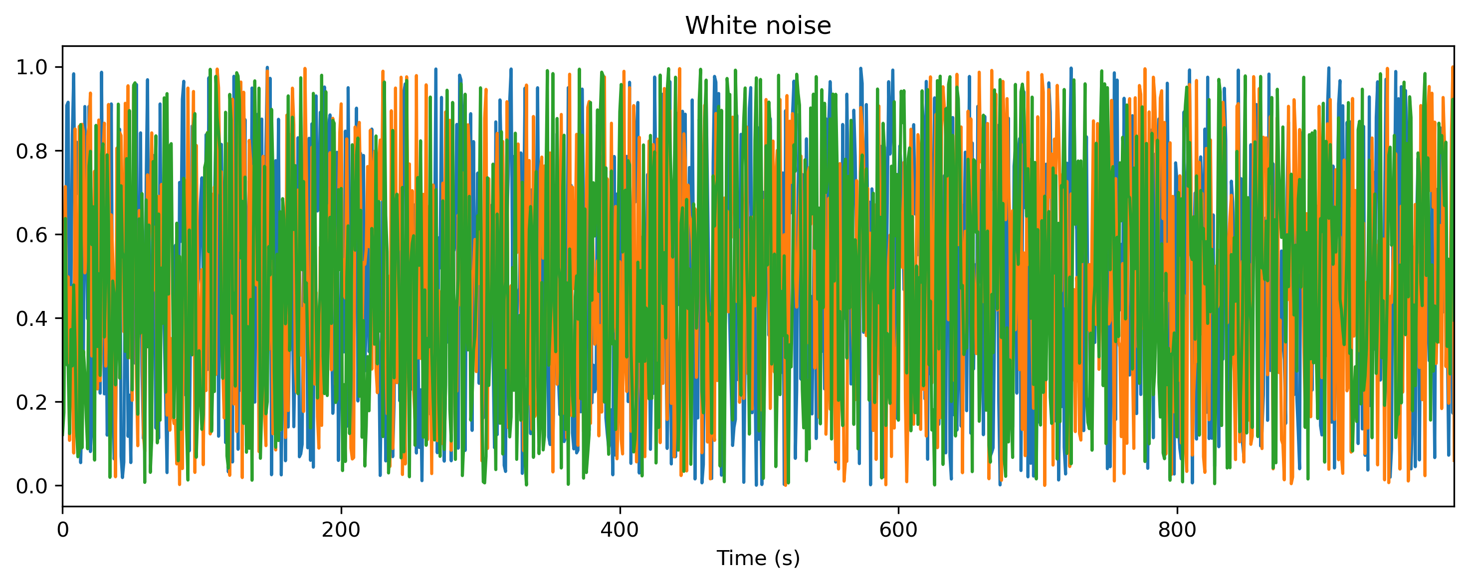
Input: periodic TSContinuous object `White noise` from t=0.0 to 1000.0. Samples: 1000. Channels: 3

Output: non-periodic TSContinuous object `Output samples` from t=0.0 to 1000.0. Samples: 1000. Channels: 7

Converting a low-level API Module to a high-level API TimedModule

You may also want to convert a low-level Module subclass into a high-level TimedModule object. Rockpool provides a convenient wrapper to do so, with TimedModuleWrapper, also accessed by the Module.timed() method.

# - Import the converter class
from rockpool.nn.modules.timed_module import TimedModuleWrapper
from rockpool.nn.modules import RateJax

# - Generate a module and wrap as a TimedModule
mod = RateJax(4)
tmod = TimedModuleWrapper(mod)
print(tmod)

TimedModuleWrapper  with shape (4, 4) {
    RateJax '_module' with shape (4,)
} with RateJax '_module' as module

# - Use the conversion method
from rockpool.nn.modules import RateJax

# - Generate a module and wrap as a TimedModule
tmod = RateJax(4).timed()
print(tmod)

TimedModuleWrapper  with shape (4, 4) {
    RateJax '_module' with shape (4,)
} with RateJax '_module' as module

Now tmod is a standard TimedModule, and transparently passes all data and attribute accesses into the wrapped Module. Input and output data will be handled as native TimeSeries objects.

Warning

Note that recorded state data will not be wrapped as TimeSeries data, but will be returned as raw arrays.

TimedModule API reference

High-level attributes and methods provided by TimedModule

Every TimedModule provides the following attributes:

Attribute	Description
dt	The time-step used by this module for simulation
t	The current time of this module
input_type	The TimeSeries subclass that is expected by this module
output_type	The TimeSeries subclass that is produced by this module

Every TimedModule provides the following methods:

Method	Description
reset_time()	Reset the internal clock of this module and submodules
reset_all()	Reset the state and internal clock of this module and submodules

TimedModule provides the following internal convenience methods to assist developers:

Method	Description
_prepare_input()	Rasterise the input for this module, to set up for evolution
_gen_time_trace()	Generate a time trace for use in building a time series
_gen_timeseries()	Convert an output rasterised array into a time series object to return from the evolve() method

Low-level attributes and methods inherited from Module

The following attributes are inherited from the low-level Module API:

Attribute	Description
class_name	The name of the subclass
name	The attribute name that this module was assigned to. Will be None for a base-level module
full_name	The class name and module name together. Useful for printing
spiking_input	If True this module expects spiking input. Otherwise the input is real-valued
spiking_output	If True this module produces spiking output. Otherwise the module outputs floating-point values
shape	The dimensions of the module. Can have any number of entries, for complex modules. shape[0] is the input dimensionality; shape[-1] is the output dimensionality.
size_in	The number of input channels the module expects
size_out	The number of output channels the module produces

The following methods are inherited from the low-level Module API:

Method	Description
parameters()	Return a nested dictionary of module parameters, optionally restricting the search to a particular family of parameters such as weights
state()	Return a nested dictionary of module state
simulation_parameters()	Return a nested dictionary of module simulation parameters
modules()	Return a list of submodules of this module
attributes_named()	Search for and return nested attributes matching a particular name
set_attributes()	Set the parameter values for this and nested submodules
reset_state()	Reset the state of this and nested submodules
reset_parameters()	Reset the parameters of this and nested submodules to their initialisation defaults