This page was generated from docs/basics/sharp_points.ipynb. Interactive online version:

🐡 The sharp points of Rockpool 🐚

Rockpool aims to be an intuitive bridge between supervised machine learning and dynamic signal processing, hiding the complexities of the underlying dynamical systems as much as possible.

However, there are a few places where you need to consider that a Rockpool-based solution is actually a dynamical system, and not a simple stack of stateless linear algebra.

This notebook illustrates some of the sharp points that can jab you when you dip your hands into Rockpool. Our goal is to make this list disappear over time.

# - Switch off warnings
import warnings

warnings.filterwarnings("ignore")

# - Rockpool imports
from rockpool import TSContinuous

# - General imports and configuration
import numpy as np

import sys
!{sys.executable} -m pip install --quiet matplotlib
import matplotlib.pyplot as plt

%matplotlib inline
plt.rcParams["figure.figsize"] = [12, 4]
plt.rcParams["figure.dpi"] = 300

🦀 How to use sampled time series data (in)correctly in Rockpool

Time series data loaded from elsewhere probably comes in a clocked raster format. You can easily use this data in Rockpool, but there are a couple of tricky points to watch out for.

Wrong: how to generate a time base for clocked data

T = 1000
dt = 1e-3
data = np.random.rand(T)
t_start = 23.6
time_base = np.arange(t_start, t_start + len(data) * dt, dt)

This approach can sometimes lead to rounding errors such that time_base is one sample too short, especially for floating point numbers with < 64 bit precision.

The better way is to generate integer time steps, then scale and shift them:

time_base = np.arange(T) * dt + t_start

Wrong: how to define a time series from clocked data

Say we have a 20-second sample, sampled on a 100ms clock. Let’s convert this into a continuous time series:

dt = 100e-3
T = round(20 / dt)
data = np.random.rand(T)
time_base = np.arange(len(data)) * dt

ts = TSContinuous(time_base, data)
ts

non-periodic TSContinuous object `unnamed` from t=0.0 to 19.900000000000002. Samples: 200. Channels: 1

Huh? The time series is too short, it’s one dt off! But there are 200 samples…?

Time series objects don’t have an intrisic clock; you can define samples at any point in time. So TSContinuous has no way to know that you expected a 20 second duration. By default, the time series ends at the point in time where the last sample occurs. But for clocked data, you probably expected there to be an extra dt.

The correct low-level way to define the time series is to specify t_stop explicitly:

ts = TSContinuous(time_base, data, t_stop=20.0)
ts

non-periodic TSContinuous object `unnamed` from t=0.0 to 20.0. Samples: 200. Channels: 1

However, we provide a convenience method TSContinuous.from_clocked() to make this easier:

ts = TSContinuous.from_clocked(data, dt=dt)
ts

non-periodic TSContinuous object `unnamed` from t=0.0 to 20.000000000000004. Samples: 200. Channels: 1

TSContinuous.from_clocked() is the canonical way to import clocked time-series data into Rockpool. If you use from_clocked() then everything should behave as you expect it to.

🐚 Defining extents for TSEvent time series data

Event time series are represented in Rockpool using the TSEvent class, which represents events as occuring at discrete moments in time, on one of a number of channels. This is different from an “event raster” representation, where events are placed into discrete time bins, and the temporal resolution is limited to bin durations dt.

from rockpool import TSEvent
from matplotlib import pyplot as plt

times = [0.2, 0.8, 1.2, 1.4, 1.8, 2.2, 3.3, 3.5, 3.6, 4.2, 4.8, 5.2, 5.8, 6.2, 6.5, 6.8]
channels = [0, 3, 3, 1, 6, 6, 3, 3, 5, 5, 4, 0, 5, 1, 1, 2]
ts = TSEvent(times, channels, t_start=0.0, t_stop=7.0)
ts.plot();

from IPython.display import Image

Image("TSEvent_to_raster.png")

The image above shows the relationship between an event time series and one possible raster representation of that time series. Note that a raster is inherently lossy — it can only represent events down to a minimum temporal resolution dt.

We can convert a TSEvent object into a raster by using the appropriately-named raster() method:

def raster(
    dt: float,
    t_start: float=None,
    t_stop: float=None,
    num_timesteps: int=None,
    channels: numpy.ndarray=None,
    add_events: bool=False,
    include_t_stop: bool=False,
) -> numpy.ndarray:

With an event raster, the time base is explicitly defined. Time proceeds from t = t_start at the beginning of the raster, and continues until t = t_start + dt * T at the end of the raster (after T time bins). If you convert a raster directly to a TSEvent object using the from_raster() method, then t_start and t_stop are inferred.

But a freshly-created TSEvent object can’t infer t_start and t_stop — we need to supply these explicitly when creating the TSEvent. If we don’t, things can get confusing:

tsBad = TSEvent(times, channels, t_stop=7.0, name="No extents 🤢🤬")
print(tsBad)

tsGood = TSEvent(times, channels, t_start=0.0, t_stop=7.0, name="With extents 😇🥰")
print(tsGood)

non-periodic `TSEvent` object `No extents 🤢🤬` from t=0.2 to 7.0. Channels: 7. Events: 16
non-periodic `TSEvent` object `With extents 😇🥰` from t=0.0 to 7.0. Channels: 7. Events: 16

Imagine you tried to evolve() a layer with the first ts — the evolve() method would probably get the evolution duration wrong.

Things would also get messy if you tried to convert the first ts to a raster(). The time bins would begin at t = 0.2 rather than t = 0.

The moral of the story is, you should always set the extents for a TSEvent, if you are creating it from a list of event times.

🐡 TimeSeries and Modules share an explicit global time base

All TimeSeries and Module objects in Rockpool are defined with a shared global time base. That means t = 0 refers to the same point in time for all objects.

This may slip you up if you play with a layer for while, evolving with some input time series, and expect that evolution will begin from the start of the time series data for each evolution.

# - Imports
from rockpool.nn.modules import Rate
from rockpool import TSContinuous

# - Define a Timed module with a single rate neuron
tmod = Rate(1).timed()
print("tmod:", tmod)

# - Define a time series
dt = 1e-3
data = np.sin(np.arange(0, 10, dt) / 4 * (2 * np.pi))
ts_input = TSContinuous.from_clocked(data, dt=dt)
ts_input.plot();

tmod: TimedModuleWrapper  with shape (1, 1) {
    Rate '_module' with shape (1,)
} with Rate '_module' as module

Now we evolve tmod using ts_input, and look at the result.

output_ts, _, _ = tmod(ts_input)
output_ts.plot()

[<matplotlib.lines.Line2D at 0x7fe2aefbc550>]

But if we try to evolve mod again in the same way, we recieve an error.

tmod(ts_input);

---------------------------------------------------------------------------
ValueError                                Traceback (most recent call last)
/var/folders/fj/ptcl18sd0yd8n9bm9fs_qtrc0000gn/T/ipykernel_10376/2584389186.py in <module>
----> 1 tmod(ts_input);

~/SynSense Dropbox/Dylan Muir/LiveSync/Development/rockpool_GIT/rockpool/nn/modules/timed_module.py in __call__(self, *args, **kwargs)
    725                 record_state (dict): If the argument ``record`` is ``True``, ``record_state`` must contain a dictionary of the recorded states o this and all sub-modules during evolution. Otherwise it may be an empty dict.
    726         """
--> 727         return self.evolve(*args, **kwargs)
    728
    729     @property

~/SynSense Dropbox/Dylan Muir/LiveSync/Development/rockpool_GIT/rockpool/nn/modules/timed_module.py in _evolve_wrapper(self, ts_input, duration, num_timesteps, kwargs_timeseries, record, *args, **kwargs)
    289         """
    290         # - Determine number of timesteps
--> 291         num_timesteps = self._determine_timesteps(ts_input, duration, num_timesteps)
    292
    293         # - Call wrapped evolve

~/SynSense Dropbox/Dylan Muir/LiveSync/Development/rockpool_GIT/rockpool/nn/modules/timed_module.py in _determine_timesteps(self, ts_input, duration, num_timesteps)
    344                     duration = ts_input.t_stop - self.t
    345                     if duration <= 0:
--> 346                         raise ValueError(
    347                             self.full_name
    348                             + "Cannot determine an appropriate evolution duration."

ValueError: TimedModuleWrapper Cannot determine an appropriate evolution duration. 'ts_input' finishes before the current evolution time.

This is because the internal time of the layer is after the defined times of the timeseries.

There are several possibilities to resolve this issue, one of which is simply delaying ts_input on creation by using the t_start argument to from_clocked():

ts_input = TSContinuous.from_clocked(data, dt=dt, t_start=tmod.t)
print("ts_input:", ts_input)
output, _, _ = tmod(ts_input)

ts_input: non-periodic TSContinuous object `unnamed` from t=10.0 to 20.000000000000004. Samples: 10000. Channels: 1

or by using the TSContinuous.start_at() or TSContinuous.delay() methods when calling evolve():

# - Using `.start_at()`
tmod(ts_input.start_at(tmod.t))

# - Using `.delay()`
tmod(ts_input.delay(tmod.t - ts_input.t_start));

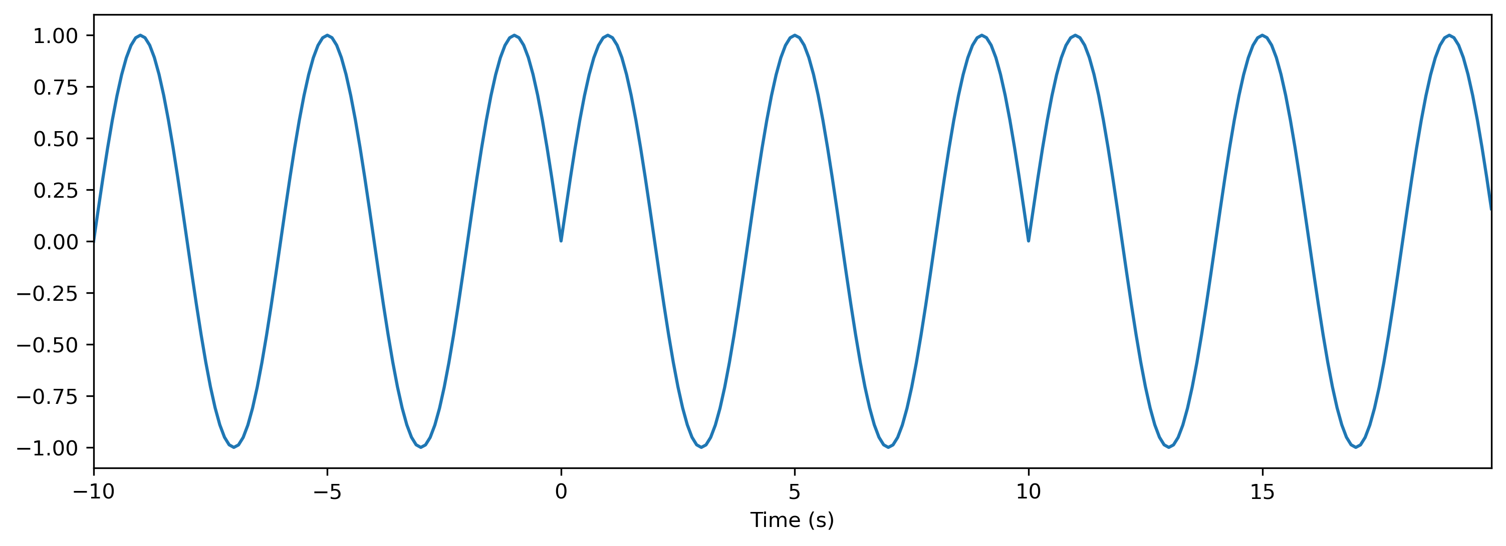
The final possibility is to specify that the time series is periodic, using the periodic = True flag to TSContinuous.from_clocked(). The time series will then be defined over all time:

ts_input = TSContinuous.from_clocked(data, dt=dt, periodic=True)
ts_input.plot(np.arange(-10, 20, 0.1));

and we can evolve as we like:

tmod(ts_input)
tmod(ts_input);

🦀 Modules in Rockpool are dynamical systems, and don’t get reset implicitly

Neurons and modules in Rockpool behave quite differently from standard ANNs. They are intrinsically stateful, even in the absence of explicit recurrent connectivity. Single neurons have an internal state, which evolves dynamically over time following a set of differential equations.

Standard ANNs are stateless, meaning that each frame or sample is processed completely independently. Recurrent ANNs or LSTMs are often implicitly reset at the start of each trial. Neurons in Rockpool are only ever reset explicitly using nn.modules.Module.reset_state().

An explicit reset could become important during training, to ensure that a network’s response to a trial is not contaminated by the response to the previous trial.