This page was generated from docs/devices/analog-frontend-example.ipynb. Interactive online version:

Using the analog frontend model

In this notebook we will show how to use the analog frontend model for Xylo. To that end, we will make use of a very simple example - we will generate a one dimensional chirp signal of increasing frequency and process that with the devices.xylo.syns61201.AFESim.

# - Image display
from IPython.display import Image

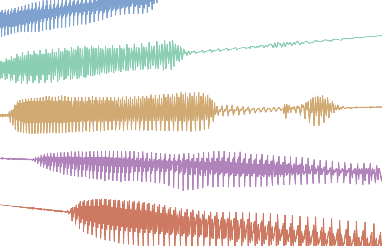
Image("images/vowels-audio-splash.png")

# - Switch off warnings
import warnings

warnings.filterwarnings("ignore")

# - Import numpy
import numpy as np
import scipy as sp

# - Import the plotting library
import sys
!{sys.executable} -m pip install --quiet matplotlib
import matplotlib.pyplot as plt

%matplotlib inline
plt.rcParams["figure.figsize"] = [16, 10]
plt.rcParams["figure.dpi"] = 300

# - Rich printing
try:
    from rich import print
except:
    pass

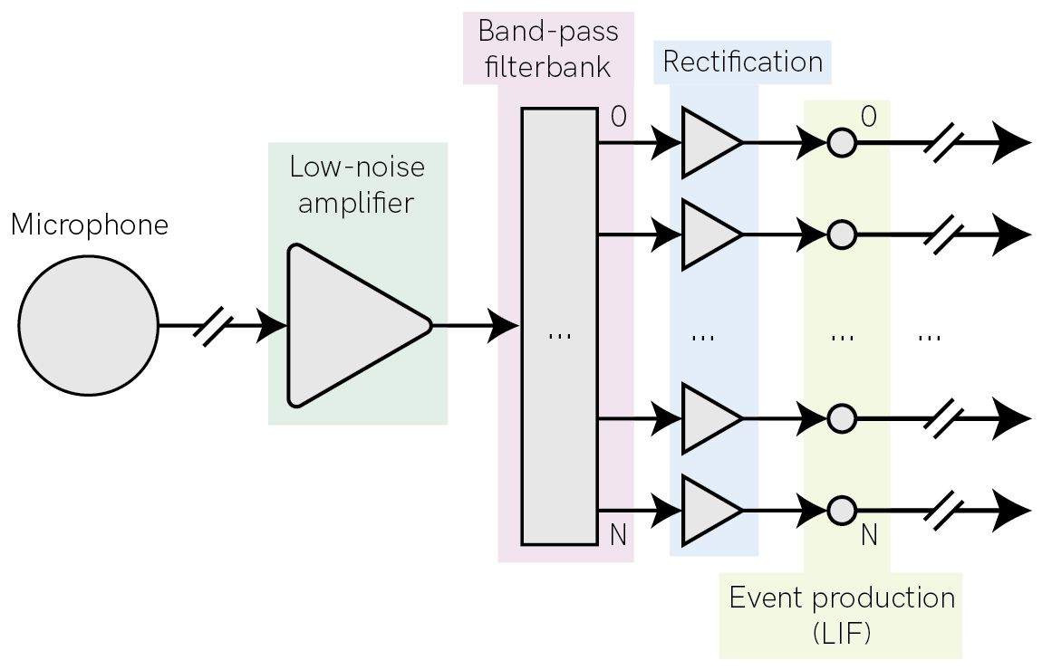
The audio front-end module

Rockpool provides a simulation of an analog front-end that performs asynchronous signal-to-event conversion. This module provides a convenient way to convert audio and other wide-band signals to events for further processing.

The AFESim Rockpool module is a simulation of harware designed for audio-to-event conversion by SynSense. AFESim realistically simulates mismatch and noise present in the physical module, and so can be used for data augmentation.

The stages of the model are shown below. The principle is to provide a filter-bank of Butterworth band-pass filters, followed by rectification and event production via a spiking LIF neuron membrane.

AFESim provides many parameters to tune the frequency range, filter quality, number of channels etc. See the API reference for AFESim for more information.

Image("images/audio-front-end.png")

Parameter definition and initialization

First, let’s define all parameters for the devices.xylo.syns61201.AFESim module and initialize it.

Some parameters are needed to be set for initialization as they are commonly used, but there are many more hidden parameters which must be set after initialization if needed.

We will see what the parameters mean in the process of this notebook.

# - import AFE
from rockpool.devices.xylo.syns61201 import AFESim

# - AFE parameters

fs = 110e3                          # The sampling frequency of the input, in Hz
raster_period = 10e-3               # The output rasterisation time-step in seconds
max_spike_per_raster_period = 15    # Maximum number of events per output time-step

add_noise = True                    # Enables / disables simulated noise generated by the AFE
add_offset = True                   # Add mismatch offset to each filter
add_mismatch = True                 # Add simualted mismatch to filter parameters
seed = None                         # Seed for mistmatch generation

# - Initialize the AFE simulation, and convert it to a high-level `TimedModule`

afe = AFESim(
        fs = fs,
        raster_period = raster_period,
        max_spike_per_raster_period = max_spike_per_raster_period,
        add_noise = add_noise,
        add_offset = add_offset,
        add_mismatch = add_mismatch,
        seed = seed,
).timed()

Input generation

For demonstation purposes we generate an artificial chirp signal of increasing frequency to be processed by the AFE.

from rockpool.timeseries import TSContinuous

# create chrip
T = 1000e-3
f0 = 50.0
f1 = 8000.0
dt = 1 / fs
chirp_amp = 112e-3
noise_amp = 0.5e-3
offset = 0.0
times = np.arange(0, T, dt)
inp = chirp_amp * sp.signal.chirp(times, f0, T, f1, method="logarithmic") + offset
inp += noise_amp * np.random.normal(size=len(times))

inp_ts = TSContinuous.from_clocked(inp, dt=dt, periodic=True, name="Chirp input")
inp_ts

periodic TSContinuous object `Chirp input` from t=0.0 to 1.0. Samples: 110000. Channels: 1

The signal has a duration of 1 second and the frequencies in this chirp range from 50 to 8000 Hz. We use a logarithmic chirp, since the distribution of filters is also logarithmic, so this helps for visualisation.

Then we can do a short time fourier transformation (STFT) to see the change in frequencies in the signal.

# - Plot the input signal
fig = plt.figure()
ax = fig.add_subplot(211)
inp_ts.plot()
# ax.set_xlim([0, 100e-3])

# - Plot a spectrogram
ax = fig.add_subplot(212)
ax.specgram(inp, Fs=fs)
ax.set_ylim([0, 8000])
ax.set_ylabel("Frequency (Hz)")
ax.set_xlabel("Time (s)")
ax.set_title("Spectrogram");

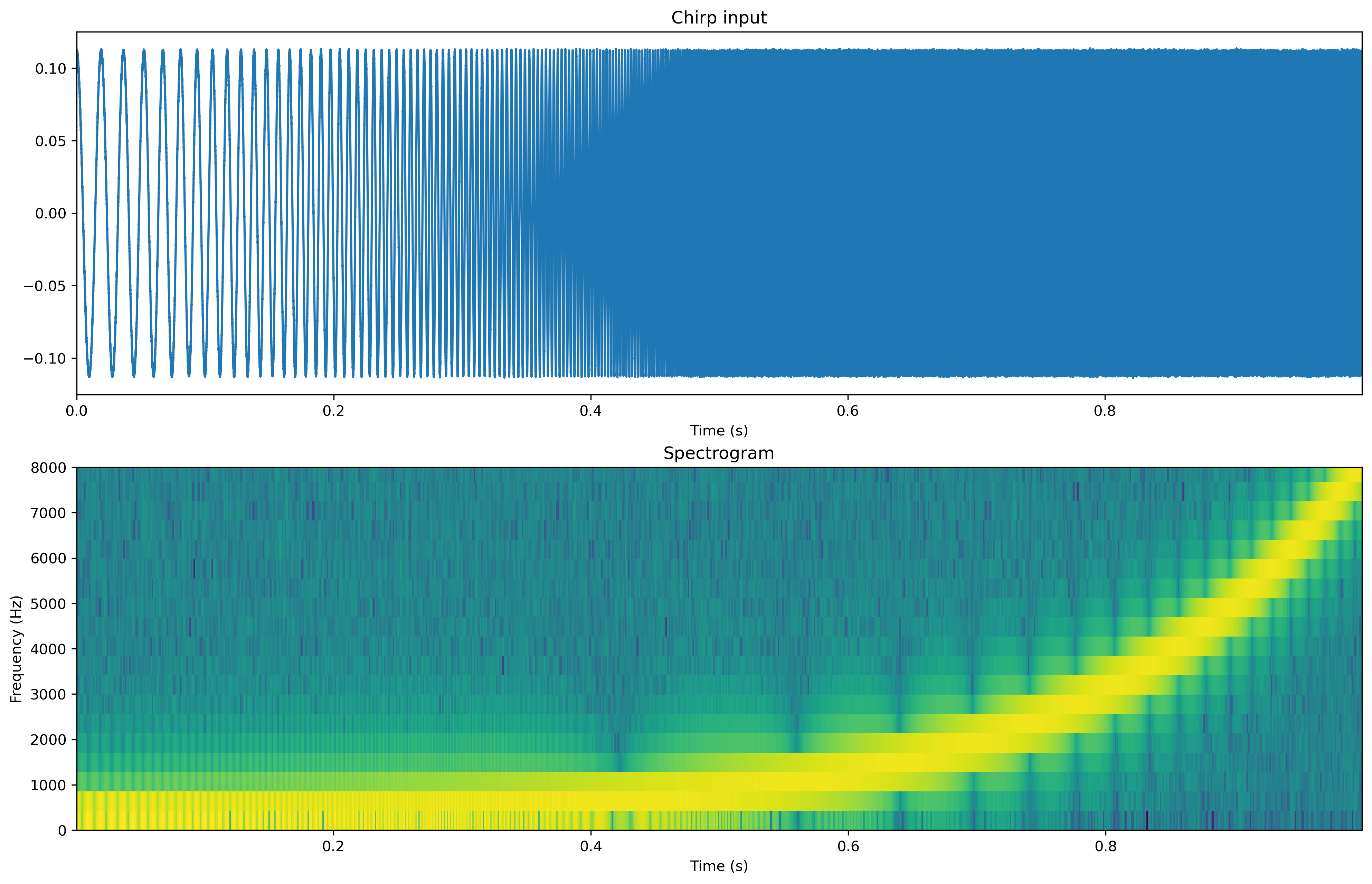
In the first panel we see the expected increase in frequency in the raw data. In the second panel we see that for increasing time slices the dominant frequencies components are increasing to 8kHz.

Now let’s see how the AFE processes this data and plot the different stages.

The stages contain:

- Low-noise amplification
- Band-pass filters
- Full-wave rectification
- Spike conversion

filt_spikes, state, rec = afe(inp_ts, record=True)

fig = plt.figure(figsize=(16, 16))
ax = fig.add_subplot(511)
inp_ts.plot()
ax.set_xticks([])
ax.set_xlabel("")

ax = fig.add_subplot(512)
rec["LNA_out"].plot()
ax.set_xticks([])
ax.set_xlabel("")

ax = fig.add_subplot(513)
rec["BPF"].plot()
ax.set_xticks([])
ax.set_xlabel("")

ax = fig.add_subplot(514)
rec["rect"].plot()
ax.set_xticks([])
ax.set_xlabel("")

ax = fig.add_subplot(515)
plt.imshow(
    filt_spikes.raster(dt=10e-3, add_events=True).T, aspect="auto", origin="lower"
)
ax.set_xlabel("Time (s)")
ax.set_ylabel("Output channel")
ax.set_title("Spiking output");

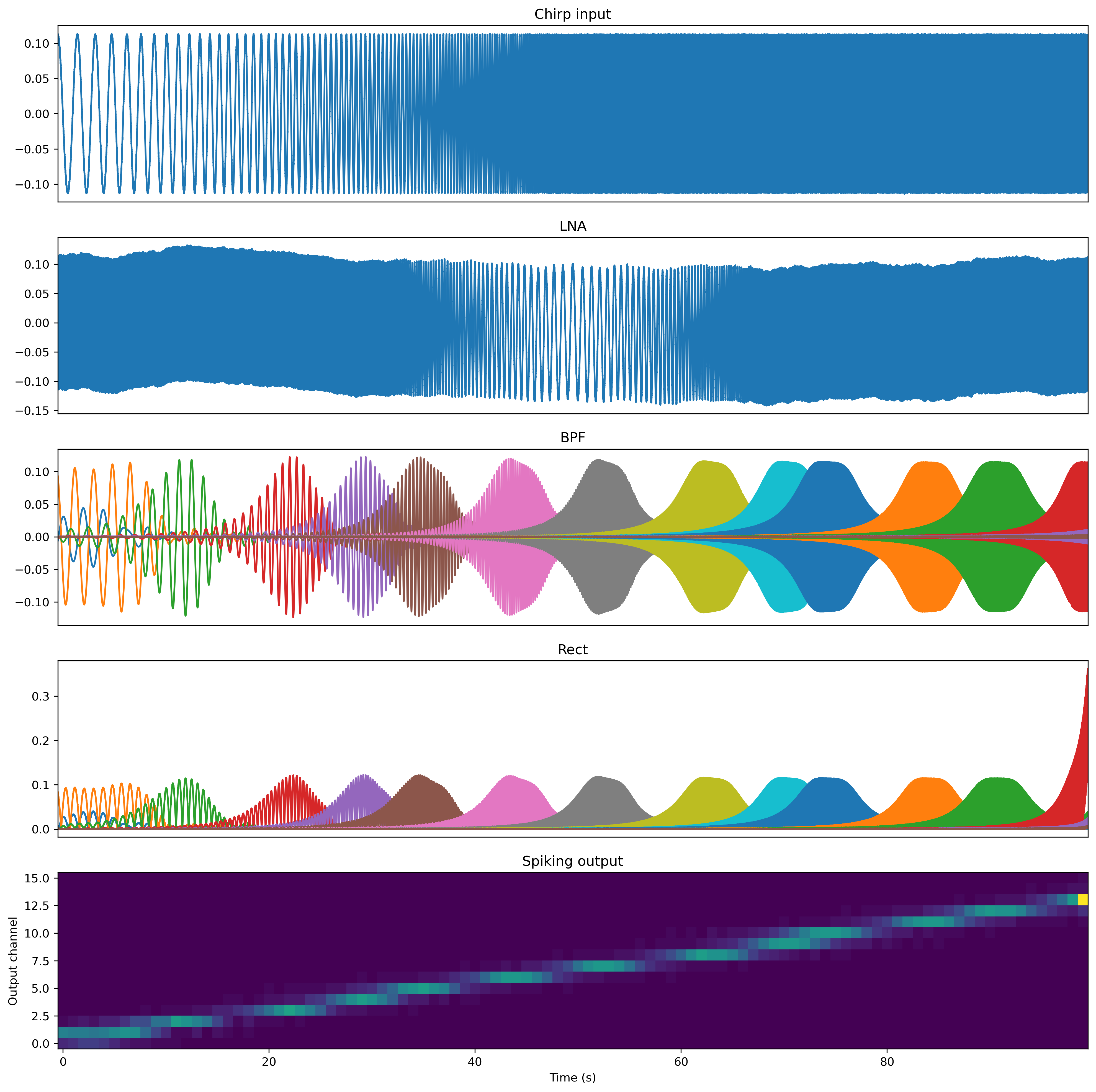
In this previous plot we can see many things. Let’s go through it piece by piece.

Input

The first panel is simply the raw input signal.

LNA

The low-noise amplifier provides normalisation and pre-amplification of the input signal, and simulates the distortion and nonlinearity present in the HW.

BPF

The bandpass filter get active in the sequence of their center frequency. You can also see that their center frequency is logarithmically distributed. The center frequency is calculated using this equation:

\(fc_i = fc_{i-1} f_\mathrm{factor}^i + fc_\mathrm{mismatch}\)

Also, the width of the filter is scaled with its center frequency. This can be manipulated using the Q factor.

Rectification

The rectification corresponds to an abs operation but is also subject to noise.

Spike conversion

As can be seen in the last panel, the different channels emit spikes corresponding to the center frequencies of their band-pass filters.

The spike conversion is done by charging a capacitor with a current corresponding to the output of the full-wave recifier. If the capacitor reaches a threshold, a spike is produced. As the capacitor is rather small on the hardware, the spike rate can get very high. The solution was to use a digital counter. The digital counter allows only every nth spike to pass and drops the rest. n can be set using the digital_counter parameter

The capacitor is subject to leak, which can be set with the leakage parameter. It can be used to lower the impact of the noise floor. If the leak is high, small background noise does not lead to threshold crossing. Try it, if the leak is reduced, the noise generated by the AFE get’s visible in the spiking output.