This page was generated from docs/tutorials/sgd_recurrent_net.ipynb. Interactive online version:

∇ Gradient descent training of a rate-based recurrent network

This tutorial demonstrates using Rockpool and a Jax-accelerated rate-based recurrent module to perform gradient descent training of all network parameters. The result is a trained dynamic recurrent network with long memory, optimised to perform a signal generation task.

Requirements

This example requires the Rockpool package from SynSense, as well as jax and its dependencies.

# - Ignore warnings
import warnings

warnings.filterwarnings("ignore")

# - Imports and boilerplate
from rockpool import TimeSeries, TSContinuous
from rockpool.nn.modules import RateJax, LinearJax
from rockpool.nn.combinators import Sequential
from rockpool.parameters import Constant
from tqdm import tnrange
from tqdm.autonotebook import tqdm

# - Numpy
import numpy as np
import numpy.random as npr

# - Matplotlib
import sys
!{sys.executable} -m pip install --quiet matplotlib
import matplotlib.pyplot as plt

%matplotlib inline
plt.rcParams["figure.figsize"] = [12, 4]
plt.rcParams["figure.dpi"] = 300

# - Pretty printing
try:
    from rich import print
except:
    pass

Triggered signal-generation task

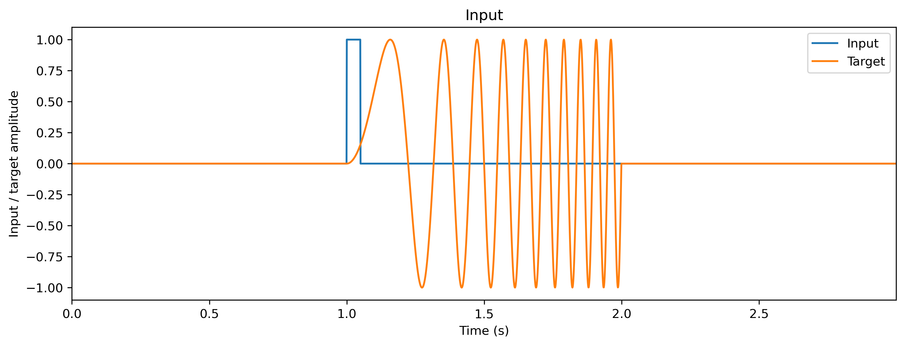
We will use a pulse-to-chirp task as a demonstration. The recurrent network receives a short pulse, and must respond by generating a chirp signal (a sinusoid increasing in frequency over time). This task is difficult, as no input is present for most of the time, and so considerable temporal memory is required in the network.

You can adjust the parameters of the input by changing the number of repeats num_repeats, the duration of the input pulse pulse_duration, and the maximum frequency reached by the chirp chirp_freq_factor in the cell below. Shorter pulses and higher chirp frequencies make the problem more difficult. More repeats make BPTT learning more difficult, by forcing gradients to be accumulated over more time steps.

You can also adjust the time step dt, which makes learning slower (more time points evaluated per trial), but which permits shorter time constants to be used in the network. For numerical stability, time constants must be at least 10*dt.

# - Define input and target signals
num_repeats = 1
pulse_duration = 50e-3
chirp_freq_factor = 10
padding_duration = 1
chirp_duration = 1
dt = 1e-3

# - Build chirp and trigger signals
chirp_end = int(np.round(chirp_duration / dt))
chirp_timebase = np.linspace(0, chirp_end * dt, chirp_end)
chirp = np.atleast_2d(
    np.sin(chirp_timebase * 2 * np.pi * (chirp_timebase * chirp_freq_factor))
).T
trigger = np.atleast_2d(chirp_timebase < pulse_duration).T

# - Add padding
padding = np.zeros((int(np.round(padding_duration / dt)), 1))
chirp = np.vstack((padding, chirp, padding))
trigger = np.vstack((padding, trigger, padding))

# - Build a time base
num_samples = (chirp_end + len(padding) * 2) * num_repeats
timebase = np.linspace(0, num_samples, num_samples + 1)
timebase = timebase[:-1] * dt

# - Replicate out inputs and target signals
input_t = np.tile(trigger * 1.0, (num_repeats, 1))
target_t = np.tile(chirp, (num_repeats, 1))

# - Generate time series objects
ts_input = TSContinuous.from_clocked(input_t, dt=dt, periodic=True, name="Input")
ts_target = TSContinuous.from_clocked(target_t, dt=dt, periodic=True, name="Target")

# - Plot the input and target signals
plt.figure()
ts_input.plot()
ts_target.plot()
plt.xlabel("Time (s)")
plt.ylabel("Input / target amplitude")
plt.legend();

Network model

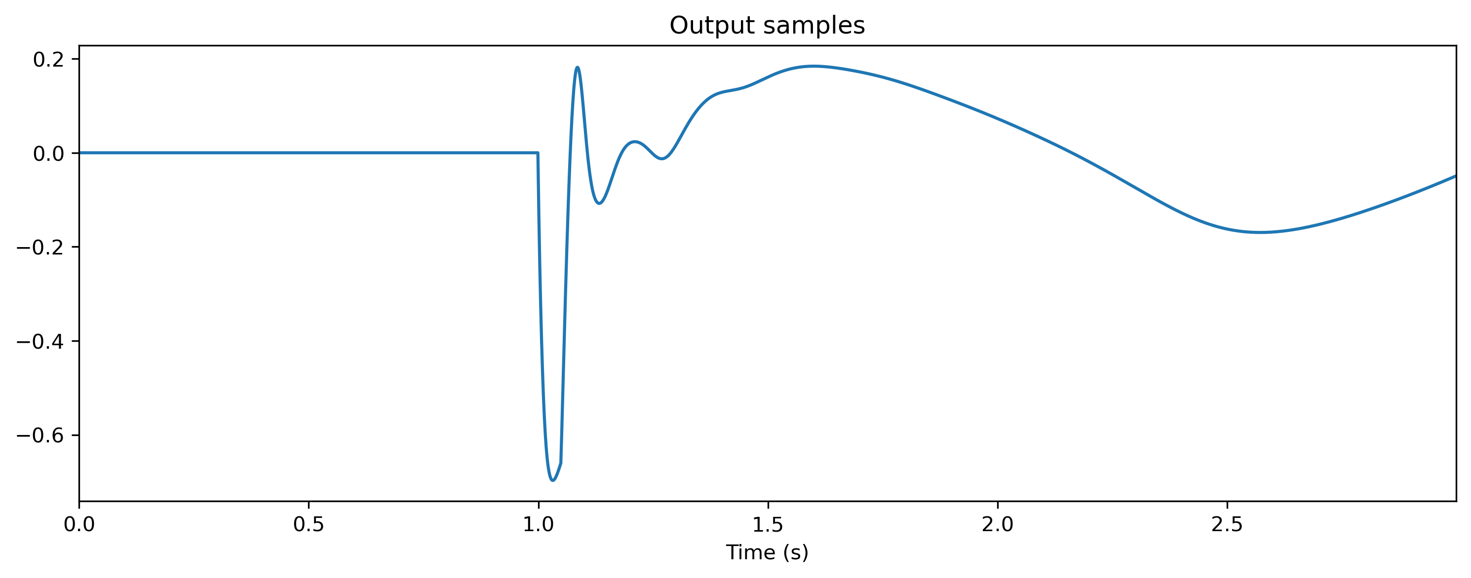
We will define a ReLU recurrent module, with a single input and a single output channel, and with a chosen number of units in the recurrent layer nResSize. Larger reservoirs take longer to train, but perform the task to higher accuracy. We’ll use the Rockpool modules RateJax and LinearJax, and the combinator Sequential

The dynamics of a unit \(j\) in the recurrent layer is given by

\[\tau_j\frac{\textrm{d}{x_j}}{\textrm{d}t} + {x_j} = W_r \cdot f(\textbf{x}) + b_j + i_j + \sigma\zeta_j(t)\]

where \(\tau_j\) is the time constant of the unit (tau); \(W_r\) is the \(N \times N\) weight matrix defining the recurrent connections; \(\textbf{x}\) is the vector of recurrent layer activities (w_rec); \(f(x)\) is the neuron transfer function \(\tanh(x)\); \(b_j\) is the bias input of the unit (bias); \(i_j\) is the external input to the unit; and \(\sigma\zeta_j(t)\) is a white noise Wiener process with standard deviation \(\sigma\) (noise_std) after 1s.

External input is weighted such that \(\textbf{i} = W_i \cdot i(t)\), where \(W_i\) is the external input weight matrix (w_in) and \(i(t)\) is the external input function.

The output of the reservoir is also weighted such that \(z = W_o \cdot \textbf{x}\), where \(W_o\) is the output weight matrix (w_out). The goal of the training task is to match the reservoir output \(\hat{z}\) with a target signal \(z^*\).

Weight initialisation doesn’t seem to matter too much in this process; gradient descent does a good job even when weights are initially zero. Here we use a standard initialisation with unit spectral radius for the recurrent weights.

You can change the activation function to one of 'tanh' or 'relu'. You can also define your own, but must use jax.numpy to do so.

# - Define the reservoir parameters
nResSize = 50
activation_func = "tanh"
noise_std = 0.1

# - Build a network
nInSize = 1
nOutSize = 1

modRNN = Sequential(
    LinearJax((nInSize, nResSize)),
    RateJax((nResSize, nResSize), has_rec=True, activation_func=activation_func, dt=dt),
    LinearJax((nResSize, nOutSize)),
).timed(dt=dt)

# - Record initial weights
w_rec0 = modRNN._module[1].w_rec
tau0 = modRNN._module[1].tau

# - Get initial output and plot
ts_output0, _, _ = modRNN(ts_input)
ts_output0.plot();

Here we use a stochastic gradient-descent optimiser “Adam” provided by Jax to optimise all network parameters.

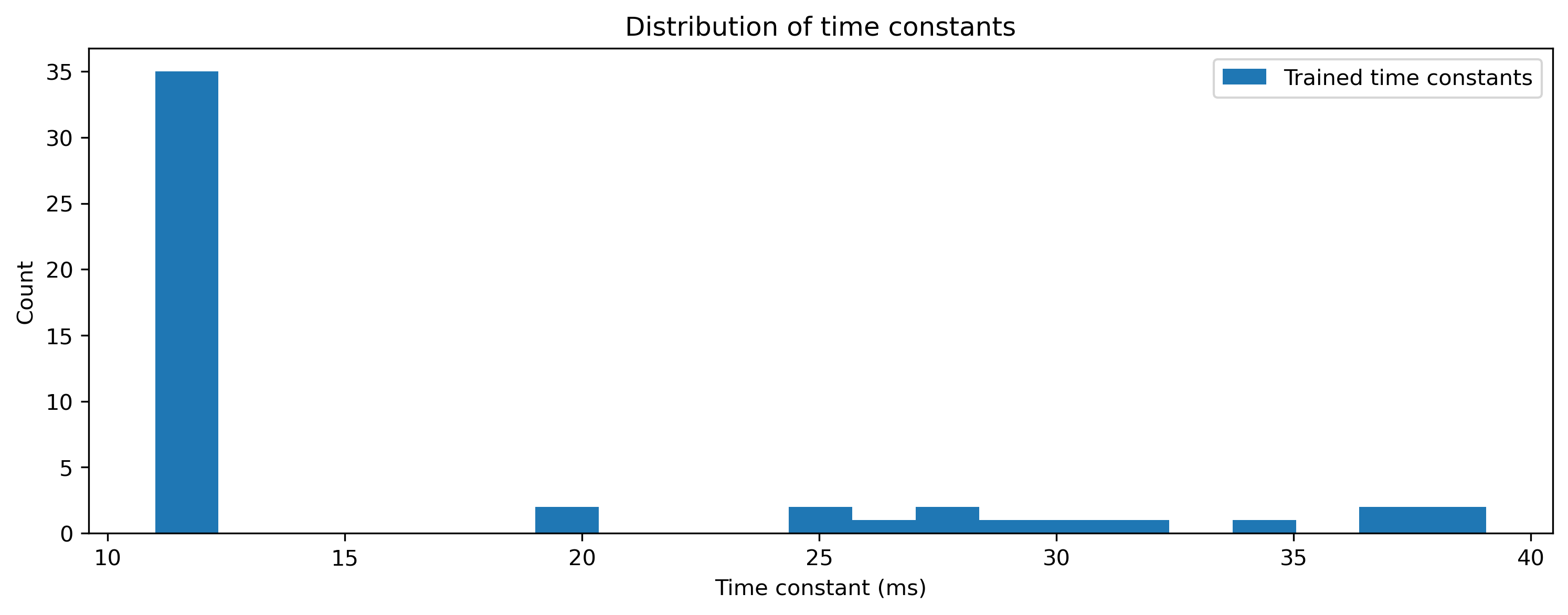
First we need to define a loss function. This will be based around the mean-squared error (MSE)between the network output and the target signal, but with an additional harsh penalty for time constants \(\\tau\) that violate a minimum bound. To impose the bounds we use the Rockpool convenience functions bounds_cost() and make_bounds(); to compute MSE we use the loss component mse(); both are available from the Rockpool package via jax_loss.

# - Import the convenience functions
from rockpool.training.jax_loss import bounds_cost, make_bounds

# - Generate a set of pre-configured bounds
lower_bounds, upper_bounds = make_bounds(modRNN.module.parameters())
print("lower_bounds: ", lower_bounds, "upper_bounds: ", upper_bounds)

lower_bounds:  {'0_LinearJax': {'weight': -inf}, '1_RateJax': {'bias': -inf, 'tau': -inf, 'threshold': -inf, 'w_rec': -inf}, '2_LinearJax': {'weight': -inf}} upper_bounds:  {'0_LinearJax': {'weight': inf}, '1_RateJax': {'bias': inf, 'tau': inf, 'threshold': inf, 'w_rec': inf}, '2_LinearJax': {'weight': inf}}

# - Impose a lower bound for the time constants
lower_bounds["1_RateJax"]["tau"] = 11 * dt

# - Define a constrained MSE loss function
import rockpool.training.jax_loss as l


def loss_mse(parameters, net, inputs, target):
    # - Handle the network state — randomise or reset
    net = net.reset_state()

    # - Assign the provided parameters to the network
    net = net.set_attributes(parameters)

    # - Evolve the network to get the ouput
    output, _, _ = net(inputs)

    # - Impose the bounds
    bounds = bounds_cost(parameters, lower_bounds, upper_bounds)

    # - Regularise recurrent weights
    reg_l2 = l.l2sqr_norm(parameters["1_RateJax"]["w_rec"])

    # - Compute a loss value w.r.t. the target output
    return l.mse(output[0], target) + 10.0 * bounds + reg_l2

# - Useful imports
from copy import deepcopy
from itertools import count

# -- Import an optimiser to use and initalise it
import jax
from jax.example_libraries.optimizers import adam

# - Get the optimiser functions
init_fun, update_fun, get_params = adam(1e-4)

# - Initialise the optimiser with the initial parameters
params0 = deepcopy(modRNN.module.parameters())
opt_state = init_fun(params0)

# - Get a compiled value-and-gradient function
loss_vgf = jax.jit(jax.value_and_grad(loss_mse))

# - Compile the optimiser update function
update_fun = jax.jit(update_fun)

# - Record the loss values over training iterations
loss_t = []
grad_t = []

num_epochs = 6000

# - Loop over iterations
i_trial = count()
for _ in tqdm(range(num_epochs)):
    # - Get parameters for this iteration
    params = get_params(opt_state)

    # - Get the loss value and gradients for this iteration
    loss_val, grads = loss_vgf(params, modRNN.module, input_t, target_t)

    # - Update the optimiser
    opt_state = update_fun(next(i_trial), grads, opt_state)

    # - Keep track of the loss
    loss_t.append(loss_val)

# - Plot the loss curve over training
plt.plot(loss_t)
plt.yscale("log")
plt.xlabel("Iteration")
plt.ylabel("Loss")
plt.title("Training progress");

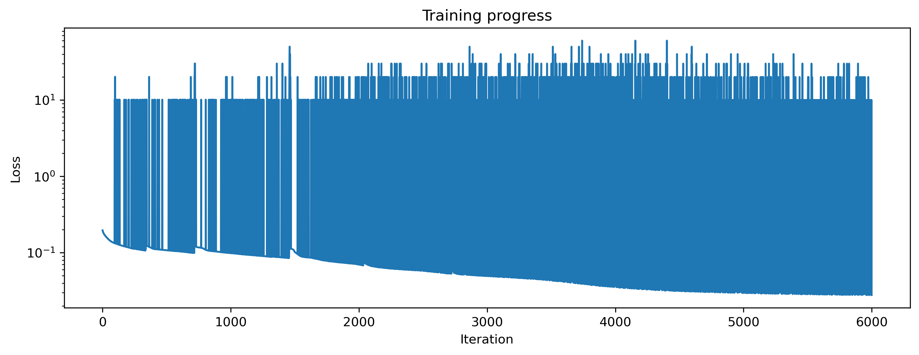
Ok, the loss has decreased to a low value. Let’s see what the network has learned!

# - Plot the output of the trained reservoir
# - Simulate with trained parameters
modRNN._module = modRNN._module.set_attributes(get_params(opt_state))
modRNN.reset_all()
ts_output, _, record_dict = modRNN(ts_input)

# - Compare the output to the target
ts_output.plot()
ts_target.plot(ts_output.times, ls="--", lw=2)
plt.legend()
plt.title("Output vs target");

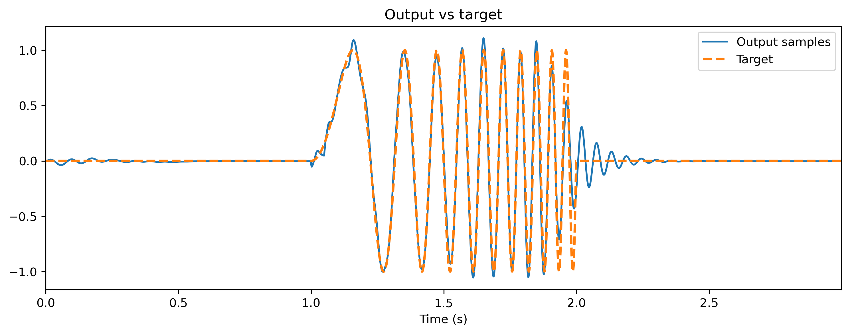
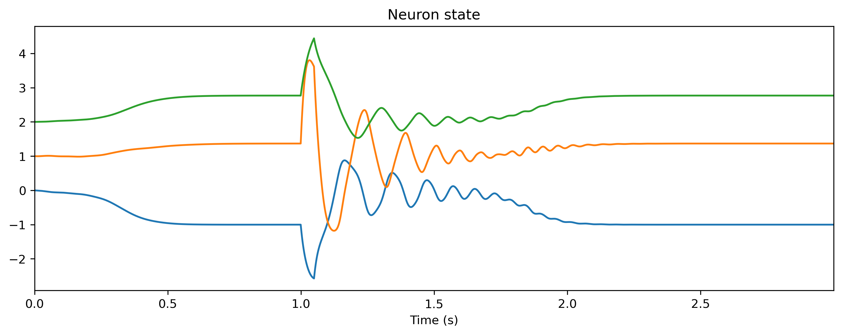
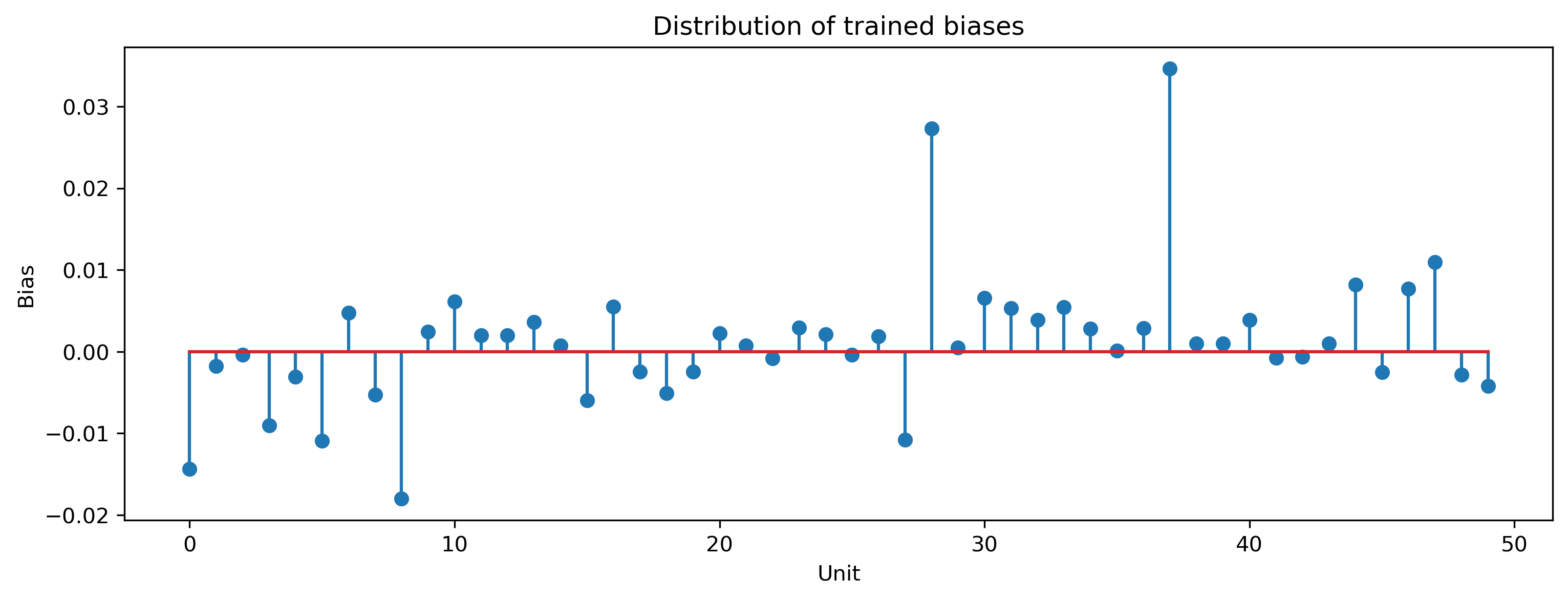
If all has gone according to plan, the output of the reservoir should closely match the target signal. We can see the effect of training by examining the distribution of network parameters below.

TSContinuous.from_clocked(
    record_dict["1_RateJax"]["x"][0], dt=dt, name="Neuron state"
).plot(skip=20, stagger=1);

# - Plot the network time constants
plt.figure()
plt.hist(modRNN._module[1].tau / 1e-3, 21)
plt.legend(["Trained time constants"])
plt.xlabel("Time constant (ms)")
plt.ylabel("Count")
plt.title("Distribution of time constants");

# - Plot the recurrent layer biases
plt.figure()
plt.stem(modRNN._module[1].bias)
plt.title("Distribution of trained biases")
plt.xlabel("Unit")
plt.ylabel("Bias");

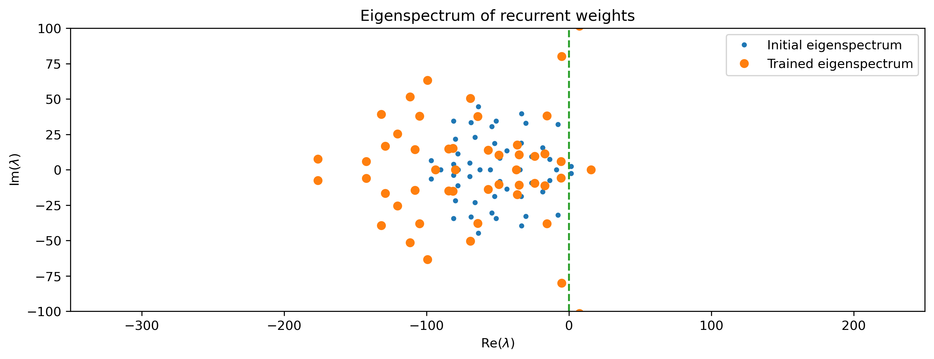
We can examine something of the computational properties of the network by finding the eigenspectrum of the Jacobian of the recurrent layer. The Jacobian \(\hat{J}\) is given by

\[\hat{J} = (\hat{W_r} - I) ./ \hat{T}\]

where \(I\) is the identity matrix, \(./\) denotes element-wise division, and \(T\) is the matrix composed of all time constants \(\hat{\tau}\) of the recurrent layer.

Below we plot the eigenvalues \(\lambda\) of \(J\). In my training result, several complex eigenvalues \(\lambda\) with real parts greater than zero are present in the trained eigenspectrum. These correspond to oscillatory modes, which are obviously useful in generating the chirp output.

# - Plot the recurrent layer eigenspectrum
J = modRNN._module[1].w_rec - np.identity(nResSize)
J = J / modRNN._module[1].tau

J0 = w_rec0 - np.identity(nResSize)
J0 = J0 / tau0

plt.figure()
eigs = np.linalg.eigvals(J)
eigs0 = np.linalg.eigvals(J0)
plt.plot(np.real(eigs0), np.imag(eigs0), ".")
plt.plot(np.real(eigs), np.imag(eigs), "o")
plt.plot([0, 0], [-100, 100], "--")
plt.legend(
    (
        "Initial eigenspectrum",
        "Trained eigenspectrum",
    )
)
plt.xlim([-350, 250])
plt.ylim([-100, 100])
plt.title("Eigenspectrum of recurrent weights")
plt.xlabel("Re($\lambda$)")
plt.ylabel("Im($\lambda$)");

The Kernel crashed while executing code in the the current cell or a previous cell. Please review the code in the cell(s) to identify a possible cause of the failure. Click <a href='https://aka.ms/vscodeJupyterKernelCrash'>here</a> for more info. View Jupyter <a href='command:jupyter.viewOutput'>log</a> for further details.

Summary

Gradient descent training does a good job of optimmising a dynamic recurrent network for a difficult task requiring significant temporal memory. jax provides a computationally efficient back-end as well as automatic differentiation of the recurrent layer. The combination in Rockpool allows us to optimise not just the weights and biases of a network, but also to adapt the neuron dynamics to a desired task.